Tutorial: a renewables-share map of Europe

For each of six big bidding zones (DE-LU, FR, ES, NL, IT-North, PL), pull one day of generation by production type, compute the share of that day's energy that came from solar + wind, and project the result onto a map. 2024-06-15 is a sunny, windy summer Saturday — a day where renewables shine.

The data layer is actual_generation_per_production_type — six calls, six cassettes, one helper to fold each into a single percentage. The presentation layer is the same Lambert Conformal Conic / Polylabel-after-projection pipeline as the 2025 EU price heat-map, so country labels land on the mainland regardless of overseas territories.

Setup

julia

using ENTSOE
using GeoMakie, CairoMakie
using GeoMakie: NaturalEarth
using GeoInterface
using Polylabel
using Proj                       # enables GeometryOps' Proj-backed extension
import GeometryOps as GO
using Dates

# Static map — no slider, no interactivity, so CairoMakie's PNG output
# is fine and avoids the heavier WGLMakie/Bonito static-export path.
CairoMakie.activate!(type = "png")

include(joinpath(pkgdir(ENTSOE), "test", "_brokenrecord_helpers.jl"))
const BR = _load_brokenrecord()
client = ENTSOEClient("PLAYBACK")

The PSR codes for "renewable, intermittent" are B16 (Solar), B18 (Wind Offshore), and B19 (Wind Onshore). Per-day share is the ratio of those rows' total energy to every row's total energy, both in MWh (since each row is a quarter-hour mean MW, multiplying by 0.25 gives MWh — that scalar cancels in the ratio so we can just sum values).

julia

const VRE_CODES = ("B16", "B18", "B19")

function vre_share(rows)
    isempty(rows) && return NaN
    total = sum(rows.value)
    iszero(total) && return NaN
    vre = sum(rows.value[in.(rows.psr_type, Ref(VRE_CODES))])
    return 100 * vre / total
end

const DAY_START = DateTime("2024-06-14T22:00")   # 2024-06-15 00:00 CET
const DAY_END   = DateTime("2024-06-15T22:00")

const ZONES = (
    (iso = "DE", eic = EIC.DE_LU,
        cassette = "tut_renewables_DE_LU_2024_06_15.yml"),
    (iso = "FR", eic = EIC.FR,
        cassette = "tut_renewables_FR_2024_06_15.yml"),
    (iso = "ES", eic = EIC.ES,
        cassette = "tut_renewables_ES_2024_06_15.yml"),
    (iso = "NL", eic = EIC.NL,
        cassette = "tut_renewables_NL_2024_06_15.yml"),
    # ENTSO-E split Italy into multiple bidding zones in 2021; we use the
    # North zone here. Natural Earth knows the country as "IT".
    (iso = "IT", eic = EIC.IT_NORTH,
        cassette = "tut_renewables_IT_NORTH_2024_06_15.yml"),
    (iso = "PL", eic = EIC.PL,
        cassette = "tut_renewables_PL_2024_06_15.yml"),
)

share_by_iso = Dict{String, Float64}()
for z in ZONES
    rows = BR.playback(z.cassette) do
        actual_generation_per_production_type(
            client, z.eic, DAY_START, DAY_END,
        )
    end
    share_by_iso[z.iso] = vre_share(rows)
end
share_by_iso

Dict{String, Float64} with 6 entries:
  "IT" => 12.7591
  "ES" => 46.5625
  "FR" => 23.6118
  "PL" => 36.262
  "DE" => 64.1429
  "NL" => 30.7908

Country polygons and projection-aware labels

This is the same recipe as the EU price map: pick the country's largest sub-polygon by geodesic area (= the mainland), reproject it into our destination CRS (Lambert Conformal Conic) with GeometryOps.reproject, run Polylabel there, reproject the pole back to (lon, lat).

julia

const PROJ_STR = "+proj=lcc +lat_1=35 +lat_2=65 +lat_0=50 +lon_0=10"
const WGS84    = "+proj=longlat +datum=WGS84"

function label_lonlat(geom)
    sub_polys = GeoInterface.geomtrait(geom) isa GeoInterface.MultiPolygonTrait ?
        collect(GeoInterface.getgeom(geom)) : [geom]
    main = argmax(sub -> GO.area(GO.Geodesic(), sub), sub_polys)
    pole = polylabel(GO.reproject(main, WGS84, PROJ_STR); rtol = 0.005)
    pt = GO.reproject(GeoInterface.Wrappers.Point(pole...), PROJ_STR, WGS84)
    return (GeoInterface.x(pt), GeoInterface.y(pt))
end

countries_fc = NaturalEarth.naturalearth("admin_0_countries", 50)

function _country_iso2(feature)
    p = feature.properties
    for key in (:ISO_A2_EH, :ISO_A2)
        v = get(p, key, nothing)
        v === nothing && continue
        v isa AbstractString && v != "-99" && return String(v)
    end
    return ""
end

plotted_iso     = String[]
plotted_geoms   = []
plotted_centers = Tuple{Float64, Float64}[]
for feat in countries_fc
    iso = _country_iso2(feat)
    haskey(share_by_iso, iso) || continue
    push!(plotted_iso, iso)
    push!(plotted_geoms, feat.geometry)
    push!(plotted_centers, label_lonlat(feat.geometry))
end
length(plotted_iso)

The map

julia

const COLORMAP    = :YlGn          # white → dark green for higher VRE share
const SHARE_RANGE = (0.0, 80.0)    # %

fig = Figure(size = (720, 640))
ax  = GeoAxis(fig[1, 1];
    dest = PROJ_STR,
    limits = ((-15, 35), (34, 72)),
    title = "VRE share of generation, 2024-06-15 (Solar + Wind)",
    xgridvisible = false, ygridvisible = false,
)

# Light backdrop: every European country.
for feat in countries_fc
    poly!(ax, feat.geometry;
        color = :grey85, strokecolor = :white, strokewidth = 0.4)
end
# Foreground: priced zones, colour by share.
for (i, iso) in enumerate(plotted_iso)
    poly!(ax, plotted_geoms[i];
        color = share_by_iso[iso],
        colormap = COLORMAP, colorrange = SHARE_RANGE,
        strokecolor = :white, strokewidth = 0.6,
        overdraw = false,
    )
end
# Percentage labels.
for (i, iso) in enumerate(plotted_iso)
    pct = share_by_iso[iso]
    text!(ax, plotted_centers[i]...;
        text = string(round(Int, pct), "%"),
        align = (:center, :center),
        fontsize = 16, color = :black,
        glowwidth = 4, glowcolor = (:white, 0.9),
        overdraw = true,
    )
end
Colorbar(fig[1, 2];
    colormap = COLORMAP, colorrange = SHARE_RANGE,
    label = "Solar + wind share, %",
)
fig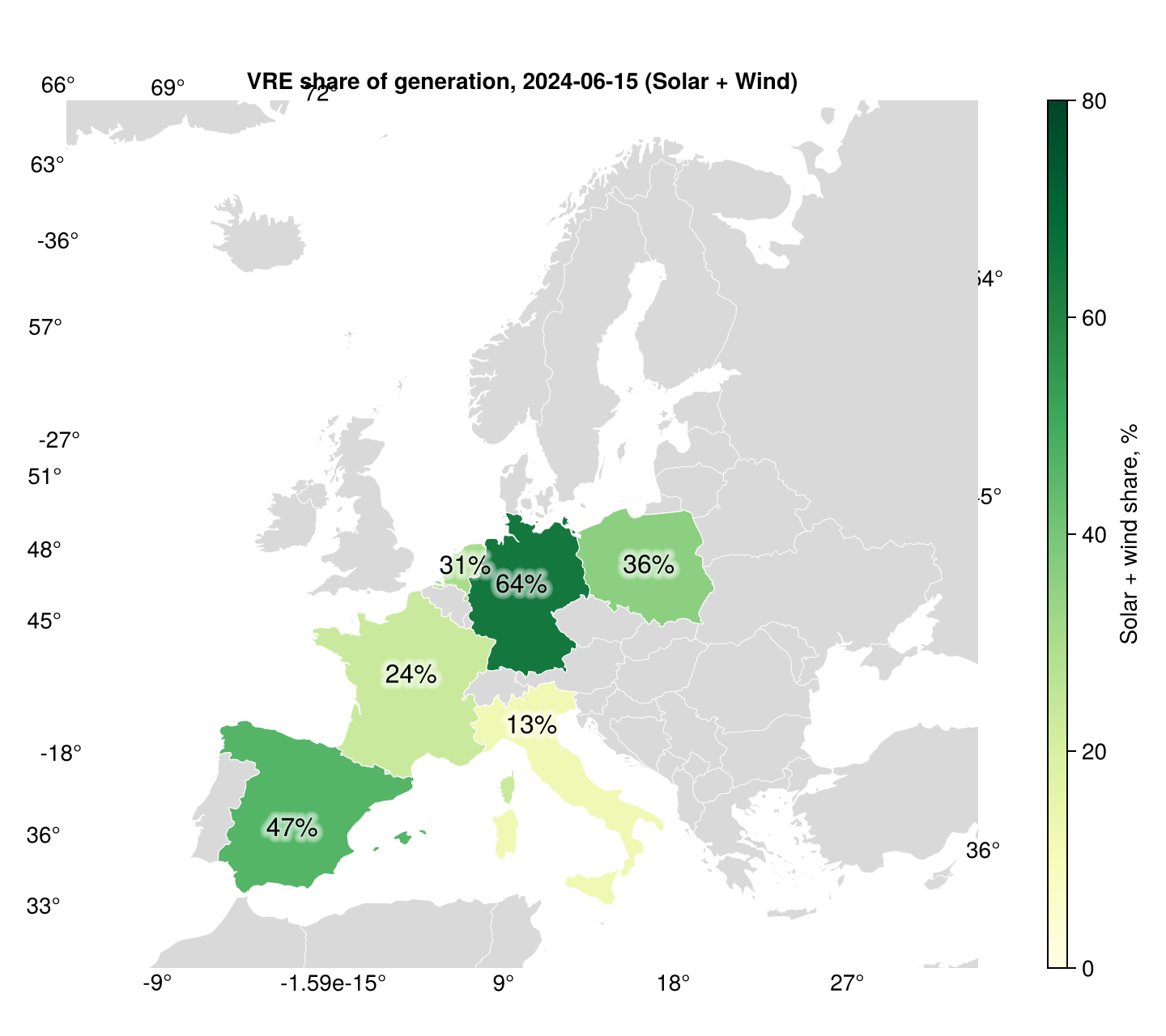

A summery weekend like this exposes the wide variation in daily VRE penetration:

Germany & Spain push past 50 % — both have huge installed PV bases that dominate a sunny day, plus DE's offshore wind staying online overnight.
France & Italy sit lower because their fleets lean nuclear (FR) and gas (IT), so the renewables denominator competes with a large fossil/nuclear baseload.
Netherlands & Poland land in the middle: NL's solar share is growing fast, while PL is still primarily coal-based.

Folding more zones in

Adding a country is one row in ZONES and one cassette in scripts/record_tutorial_cassettes.jl. Re-run that script (with a real token) and the next docs build picks up the new tile automatically. The polygon-lookup, projection, label placement, and colour bar all key off share_by_iso, so the map scales without further changes.

Where to next

For a time-varying view of a single zone's mix, see the generation mix tutorial.
For an EU-wide view of prices rather than VRE share — same GeoAxis recipe, different aggregation — see the 2025 price heat-map.

Tutorial: a renewables-share map of Europe ​

Setup ​

Zones, cassettes, and the renewables-share helper ​

Country polygons and projection-aware labels ​

The map ​

Folding more zones in ​

Where to next ​

Tutorial: a renewables-share map of Europe

Setup

Zones, cassettes, and the renewables-share helper

Country polygons and projection-aware labels

The map

Folding more zones in

Where to next