Tutorial: Austria's imbalance market

Two endpoints define the imbalance settlement market: prices (Balancing 17.1.G) and volumes (Balancing 17.1.H). Both ship as application/zip bundles of XML — the wrappers imbalance_prices and total_imbalance_volumes unzip transparently, run every member through parse_timeseries, and concatenate with vcat.

We pull the first four days of 2024 prices and one day of November 2023 volumes for Austria and look at: 2. The price time series (what the TSO paid for balancing).

3. The volume time series (how much imbalance the system absorbed).

4. The price autocorrelation — a scatter that reveals how sticky imbalance prices are minute-to-minute.

Setup

using ENTSOE
using CairoMakie
using Dates
using Statistics: mean

CairoMakie.activate!(type = "png")

include(joinpath(pkgdir(ENTSOE), "test", "_brokenrecord_helpers.jl"))
const BR = _load_brokenrecord()
# These cassettes are stored as BSON because the underlying response is
# `application/zip` — YAML can't byte-stably round-trip binary bodies.
BR.configure!(; extension = "bson")
client = ENTSOEClient("PLAYBACK")

Fetch — both zipped endpoints transparently

prices = BR.playback("tut_imbalance_prices_AT_2024.bson") do
    imbalance_prices(
        client, EIC.AT,
        DateTime("2024-01-01T00:00"), DateTime("2024-01-05T00:00");
        psr_type = PsrType.GENERATION,
    )
end
length(prices), prices[1]

(768, (time = Dates.DateTime("2024-01-01T00:00:00"), value = 45.93))

volumes = BR.playback("tut_imbalance_volumes_AT_2023.bson") do
    total_imbalance_volumes(
        client, EIC.AT,
        DateTime("2023-11-03T23:00"), DateTime("2023-11-04T23:00");
        business_type = BusinessType.BALANCE_ENERGY_DEVIATION,
    )
end
length(volumes), volumes[1]

(96, (time = Dates.DateTime("2023-11-03T23:00:00"), value = 25.62))

Imbalance prices over four days

n_p = length(prices)
# Tick every 24h (= every 96 quarter-hour samples).
p_tick = 1:96:n_p
p_lab = [Dates.format(prices.time[i], "u dd") for i in p_tick]

fig = Figure(size = (1080, 360))
ax = Axis(fig[1, 1];
    title  = "AT imbalance prices — 1–5 Jan 2024",
    xlabel = "UTC date",
    ylabel = "EUR/MWh",
    xticks = (p_tick, p_lab),
)
lines!(ax, 1:n_p, prices.value;
    color = :firebrick, linewidth = 1.0)
hlines!(ax, [mean(prices.value)];
    color = :gray60, linestyle = :dash, linewidth = 1)
fig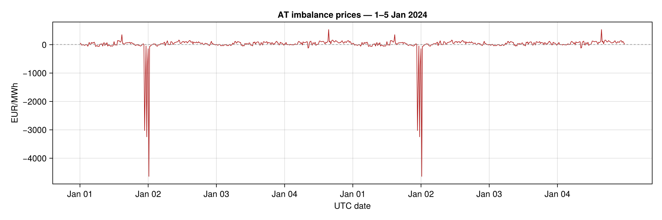

The cassette captures the New Year holiday window — prices collapsed and went negative for stretches on the 1st and 2nd, then recovered. Typical shape: low load + high renewables = TSO paying participants to consume balancing energy.

Volumes, with shading

n_v = length(volumes)
v_tick = 1:8:n_v   # every 2 h at 15-min resolution
v_lab = [Dates.format(volumes.time[i], "HH:MM") for i in v_tick]

fig2 = Figure(size = (980, 360))
ax = Axis(fig2[1, 1];
    title  = "AT total imbalance volumes — 4 Nov 2023",
    xlabel = "UTC time",
    ylabel = "MW",
    xticks = (v_tick, v_lab),
)
band!(ax, 1:n_v, zeros(n_v), volumes.value;
    color = (:steelblue, 0.4))
lines!(ax, 1:n_v, volumes.value; color = :steelblue, linewidth = 1.5)
hlines!(ax, [0]; color = :black, linewidth = 0.6)
fig2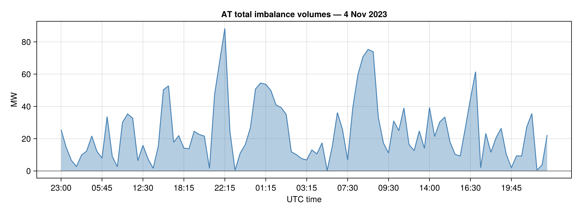

Price autocorrelation

Plotting price[t] against price[t+15min] reveals how strongly the current period predicts the next. The cloud should hug the y=x diagonal — imbalance prices are persistent.

shifted = circshift(prices.value, -1)
fig3 = Figure(size = (520, 460))
ax = Axis(fig3[1, 1];
    title  = "AT imbalance prices — autocorrelation (t vs t+15min)",
    xlabel = "Price at t (EUR/MWh)",
    ylabel = "Price at t+15min (EUR/MWh)",
)
scatter!(ax, prices.value[1:(end - 1)], shifted[1:(end - 1)];
    color = (:firebrick, 0.5), markersize = 4)
ablines!(ax, 0, 1; color = :gray60, linestyle = :dash, linewidth = 0.8)
fig3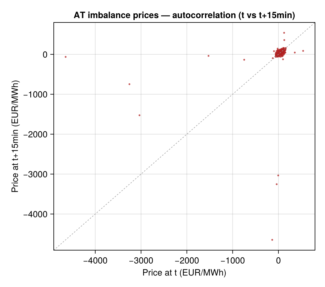

Where to next

• procured_balancing_capacity — same zipped-XML pattern; reserve-auction results per process (aFRR / mFRR / RR).

• current_balancing_state — the real-time area control error at PT1M resolution (see the balancing-state tutorial for that PT1M wiggle plot).

• aggregated_balancing_energy_bids for the bid-by-bid aFRR/mFRR/RR market data.