Tutorial: 2025 day-ahead prices across Europe
This second walkthrough fans out across most of Europe and shows the monthly mean day-ahead clearing price for every bidding zone in our EIC table over calendar year 2025 — twelve small maps in one grid, then a single full-size annual mean.
The data was pulled once with the live API (one year-long day_ahead_prices call per zone) and pre-aggregated into a small JSON fixture committed to the repo at docs/src/assets/eu_monthly_prices_2025.json. The script that produced it is scripts/record_eu_prices_2025.jl; re-run it with a valid token when 2026 closes out and the fixture refreshes itself.
Pre-aggregation is a deliberate scope choice — a year of quarter-hour prices is ~2 MB raw per zone, and we have 25 zones; baking the 12-number monthly summary keeps the docs build offline, fast, and small (~12 KB).
Loading the fixture
using ENTSOE
using JSON

const FIXTURE = joinpath(pkgdir(ENTSOE), "docs", "src", "assets",
                         "eu_monthly_prices_2025.json")
data = JSON.parsefile(FIXTURE)
year = data["year"]
zones = data["zones"]
(year = year, zone_count = length(zones))
(year = 2025, zone_count = 25)A peek at one entry — the Netherlands' twelve monthly means, January through December (EUR/MWh):
nl = zones[findfirst(z -> z["name"] == "Netherlands", zones)]
round.(Float64.(nl["monthly_eur_mwh"]); digits = 1)
12-element Vector{Float64}:
116.8
125.9
92.6
74.7
64.6
67.9
87.9
75.3
78.4
82.6
93.8
87.7Setting up the map
We use GeoMakie on top of CairoMakie to render a static PNG: country polygons (Natural Earth Admin-0 dataset) projected with Lambert Conformal Conic, coloured by their monthly mean price. Zones that overlap one country (DE_LU spans both Germany and Luxembourg, DK1 only Western Denmark, NO2/SE3 only southern halves) are coloured on the country polygon — close enough for a tutorial.
using GeoMakie, CairoMakie
using GeoMakie: NaturalEarth
using GeoInterface
using Polylabel
using Proj                       # enables GeometryOps' Proj-backed extension
import GeometryOps as GO

CairoMakie.activate!(type = "png")

# Natural Earth medium-detail country polygons. Cached after first
# fetch — subsequent runs are fast.
countries_fc = NaturalEarth.naturalearth("admin_0_countries", 50)
length(countries_fc)242Now build a lookup iso2 -> price[12] from the fixture:
price_by_iso = Dict{String, Vector{Float64}}()
for z in zones
    price_by_iso[z["iso2"]] = Float64.(z["monthly_eur_mwh"])
end
sort(collect(keys(price_by_iso)))
25-element Vector{String}:
"AT"
"BE"
"CH"
"CZ"
"DE"
"DK"
"EE"
"ES"
"FI"
"FR"
⋮
"LV"
"NL"
"NO"
"PL"
"PT"
"RO"
"SE"
"SI"
"SK"For each country polygon, decide whether it's one of our zones — we match on Natural Earth's two-letter ISO code (:ISO_A2_EH, falling back to :ISO_A2; the GeoJSON properties are Symbol-keyed). For label positions we pick the country's largest sub-polygon by geodesic area (GeometryOps.area(GeometryOps.Geodesic(), …), so mainlands beat far-flung islands on true ellipsoidal area, not degrees²), reproject it into LCC with GeometryOps.reproject, and run Polylabel.jl on the result; that lands the price label in the visual centre of each country's mainland.
const PROJ_STR = "+proj=lcc +lat_1=35 +lat_2=65 +lat_0=50 +lon_0=10"
const WGS84    = "+proj=longlat +datum=WGS84"

function label_lonlat(geom)
    sub_polys = GeoInterface.geomtrait(geom) isa GeoInterface.MultiPolygonTrait ?
        collect(GeoInterface.getgeom(geom)) : [geom]
    main = argmax(sub -> GO.area(GO.Geodesic(), sub), sub_polys)
    pole = polylabel(GO.reproject(main, WGS84, PROJ_STR); rtol = 0.005)
    pt = GO.reproject(GeoInterface.Wrappers.Point(pole...), PROJ_STR, WGS84)
    return (GeoInterface.x(pt), GeoInterface.y(pt))
end

function _country_iso2(feature)
    p = feature.properties
    for key in (:ISO_A2_EH, :ISO_A2)
        v = get(p, key, nothing)
        v === nothing && continue
        v isa AbstractString && v != "-99" && return String(v)
    end
    return ""
end

plotted_geoms   = []
plotted_iso     = String[]
plotted_centers = Tuple{Float64, Float64}[]
for feat in countries_fc
    iso = _country_iso2(feat)
    haskey(price_by_iso, iso) || continue
    push!(plotted_geoms, feat.geometry)
    push!(plotted_iso, iso)
    push!(plotted_centers, label_lonlat(feat.geometry))
end
length(plotted_iso)25A 12-month grid
Twelve mini-maps, one per month, in a 4×3 layout. A single shared Colorbar to the right of the grid keeps the colour scale honest across panels, so you can read absolute price differences just by eye.
const COLORMAP    = :magma
const PRICE_RANGE = (40.0, 160.0)
const MONTH_NAMES = ["Jan", "Feb", "Mar", "Apr", "May", "Jun",
                     "Jul", "Aug", "Sep", "Oct", "Nov", "Dec"]

fig = Figure(size = (1100, 1100))

for m in 1:12
    row = (m - 1) ÷ 3 + 1
    col = (m - 1) %  3 + 1
    ax = GeoAxis(fig[row, col];
        dest = PROJ_STR,
        limits = ((-15, 35), (34, 72)),
        title = "$(MONTH_NAMES[m]) $(year)",
        titlesize = 14,
        xgridvisible = false, ygridvisible = false,
    )
    hidedecorations!(ax)
    # backdrop: every European country light grey
    for feat in countries_fc
        poly!(ax, feat.geometry;
            color = :grey85, strokecolor = :white, strokewidth = 0.3)
    end
    # foreground: priced zones
    for (i, iso) in enumerate(plotted_iso)
        poly!(ax, plotted_geoms[i];
            color = price_by_iso[iso][m],
            colormap = COLORMAP, colorrange = PRICE_RANGE,
            strokecolor = :white, strokewidth = 0.5)
    end
end

Colorbar(fig[1:4, 4];
    colormap = COLORMAP, colorrange = PRICE_RANGE,
    label = "EUR / MWh", height = Relative(0.85))
fig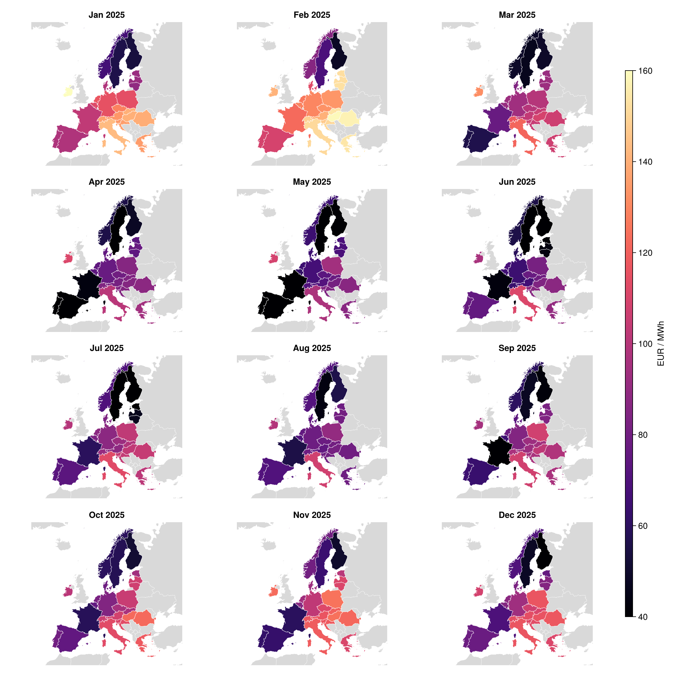
A few patterns jump out month-to-month:
Winter peak (Jan–Feb). Continental Europe sits at €110–€150 through the deep cold; Iberia is markedly cheaper as solar already contributes meaningfully.
Spring trough (Apr–Jun). Hydro, wind and solar overlap; prices drop into the €60–€80 band almost everywhere south of the Alps, while the Nordics slip into single-digit territory.
Summer rebound (Jul–Aug). South-east Europe (RO, GR, BG) pushes back up as cooling demand kicks in and hydro reservoirs draw down.
Autumn climb (Sep–Dec). Heating returns; CWE and the Iberian peninsula re-converge in the €80–€120 range by year-end.
A single annual-mean map
For the headline view, average each zone's twelve months and draw one big map with on-country price labels. Same pipeline, just one layer:
annual_by_iso = Dict(iso => sum(v) / length(v) for (iso, v) in price_by_iso)

fig2 = Figure(size = (820, 720))
ax = GeoAxis(fig2[1, 1];
    dest = PROJ_STR,
    limits = ((-15, 35), (34, 72)),
    title = "$(year) annual-mean day-ahead price",
    xgridvisible = false, ygridvisible = false,
)

for feat in countries_fc
    poly!(ax, feat.geometry;
        color = :grey85, strokecolor = :white, strokewidth = 0.4)
end
for (i, iso) in enumerate(plotted_iso)
    poly!(ax, plotted_geoms[i];
        color = annual_by_iso[iso],
        colormap = COLORMAP, colorrange = PRICE_RANGE,
        strokecolor = :white, strokewidth = 0.6)
end
for (i, iso) in enumerate(plotted_iso)
    text!(ax, plotted_centers[i]...;
        text = string(round(Int, annual_by_iso[iso])),
        align = (:center, :center),
        fontsize = 14, color = :black,
        glowwidth = 4, glowcolor = (:white, 0.9))
end
Colorbar(fig2[1, 2];
    colormap = COLORMAP, colorrange = PRICE_RANGE,
    label = "EUR / MWh")
fig2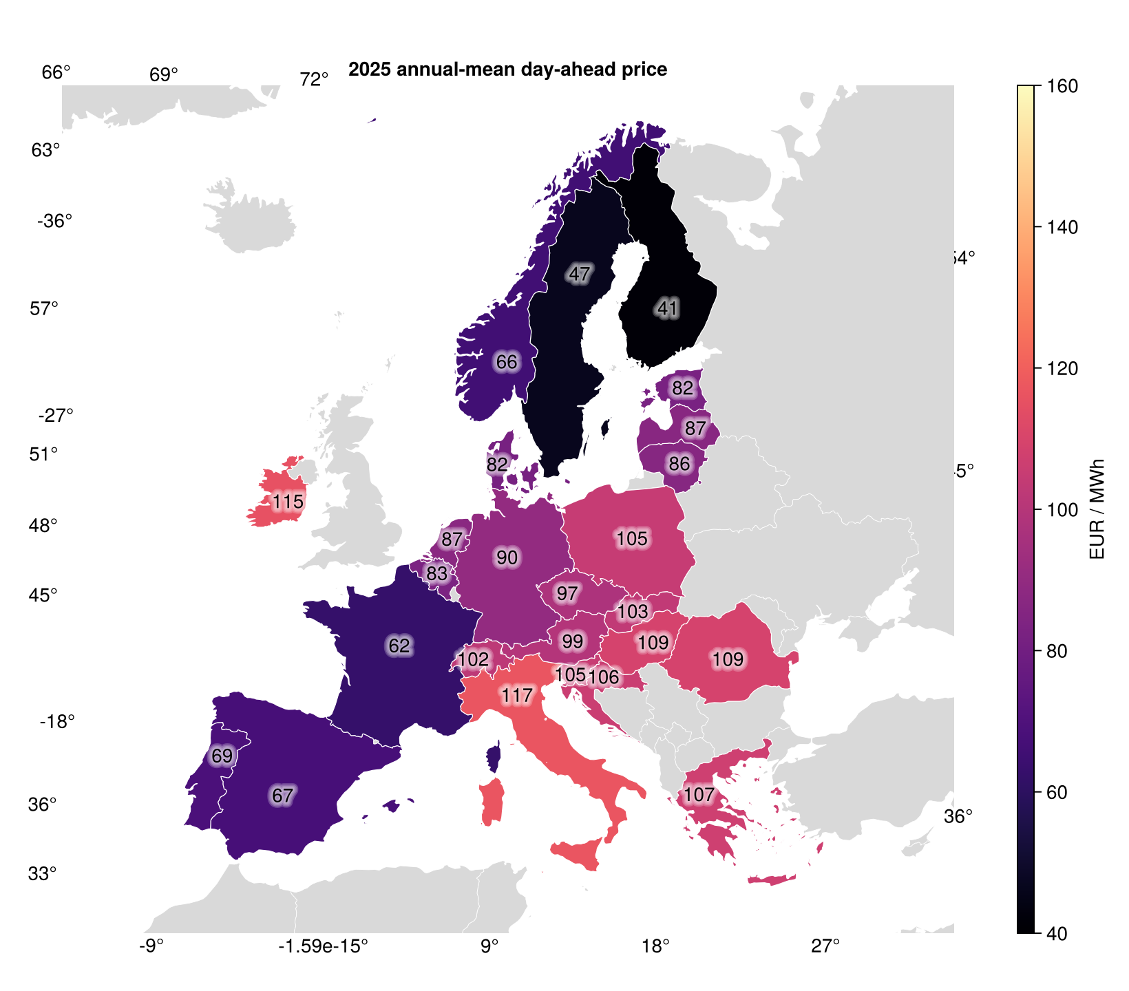
Where to next
The "first-tutorial" walkthrough —
tutorial.md— drills into the day-ahead query for one zone (NL) and parses the full quarter-hour timeseries.For the VRE-share view of the same map (solar + wind as a % of daily generation across six zones), see the renewables share map.
For more zones than the 25 we cover here, edit the
ZONEStable inscripts/record_eu_prices_2025.jland re-run; the JSON fixture picks up the additions automatically.See
day_ahead_pricesand the REST API reference for every endpoint we wrap.