Tutorial: congestion-management cost decomposition

When the day-ahead schedule produces flows the grid can't physically deliver, the TSO has three tools — they all show up under Transmission 13.1.*:

Wrapper	What it represents
redispatching_internal	Within-zone unit re-commitment
redispatching_cross_border	Between-zone re-commitment
countertrading	Energy trades that relieve a constraint
costs_of_congestion_management	Total financial cost (EUR or local CCY)

This page combines volumes from the first three with costs from the fourth to show what the TSO spent on congestion relief.

Setup

using ENTSOE
using CairoMakie
using Dates
using Statistics: mean

CairoMakie.activate!(type = "png")

include(joinpath(pkgdir(ENTSOE), "test", "_brokenrecord_helpers.jl"))
const BR = _load_brokenrecord()
client = ENTSOEClient("PLAYBACK")

Fetch the four series

Each uses a different cassette — recorded against the canonical Postman parameters that exercise each endpoint.

redispatch_internal = BR.playback("tut_redispatch_NL_2023.yml") do
    redispatching_internal(
        client, EIC.NL,
        DateTime("2023-10-31T23:00"), DateTime("2023-11-30T23:00"),
    )
end

redispatch_cross = BR.playback("transmission131_a_redispatching_cross_border.yml") do
    redispatching_cross_border(
        client, EIC.FR, EIC.AT,
        DateTime("2023-11-01T00:00"), DateTime("2023-12-01T00:00"),
    )
end

counter = BR.playback("transmission131_b_countertrading.yml") do
    countertrading(
        client, EIC.FR, EIC.ES,
        DateTime("2023-09-12T22:00"), DateTime("2023-09-13T22:00"),
    )
end

costs = BR.playback("tut_costs_BE_2022.yml") do
    costs_of_congestion_management(
        client, EIC.BE,
        DateTime("2021-12-31T23:00"), DateTime("2022-12-31T23:00"),
    )
end

(
    redispatch_internal_n = length(redispatch_internal),
    redispatch_cross_n    = length(redispatch_cross),
    counter_n             = length(counter),
    costs_n               = length(costs),
)

(redispatch_internal_n = 384, redispatch_cross_n = 44, counter_n = 53, costs_n = 36)

Costs dashboard — BE 2022

The costs cassette captures a full year of monthly cost samples for Belgium. The shape is striking — congestion costs are highly seasonal and event-driven.

fig = Figure(size = (960, 410))
ax = Axis(fig[1, 1];
    title  = "BE congestion-management cost — 2022",
    xlabel = "Month",
    ylabel = "Cost (currency varies by TSO)",
)
barplot!(ax, 1:length(costs), costs.value;
    color = costs.value,
    colormap = :acton,
    strokewidth = 0.5, strokecolor = :white)
# Y label-as-millions for readability.
ax.yticks = (
    [0, 5e5, 1e6, 1.5e6, 2e6],
    ["0", "0.5M", "1M", "1.5M", "2M"],
)
fig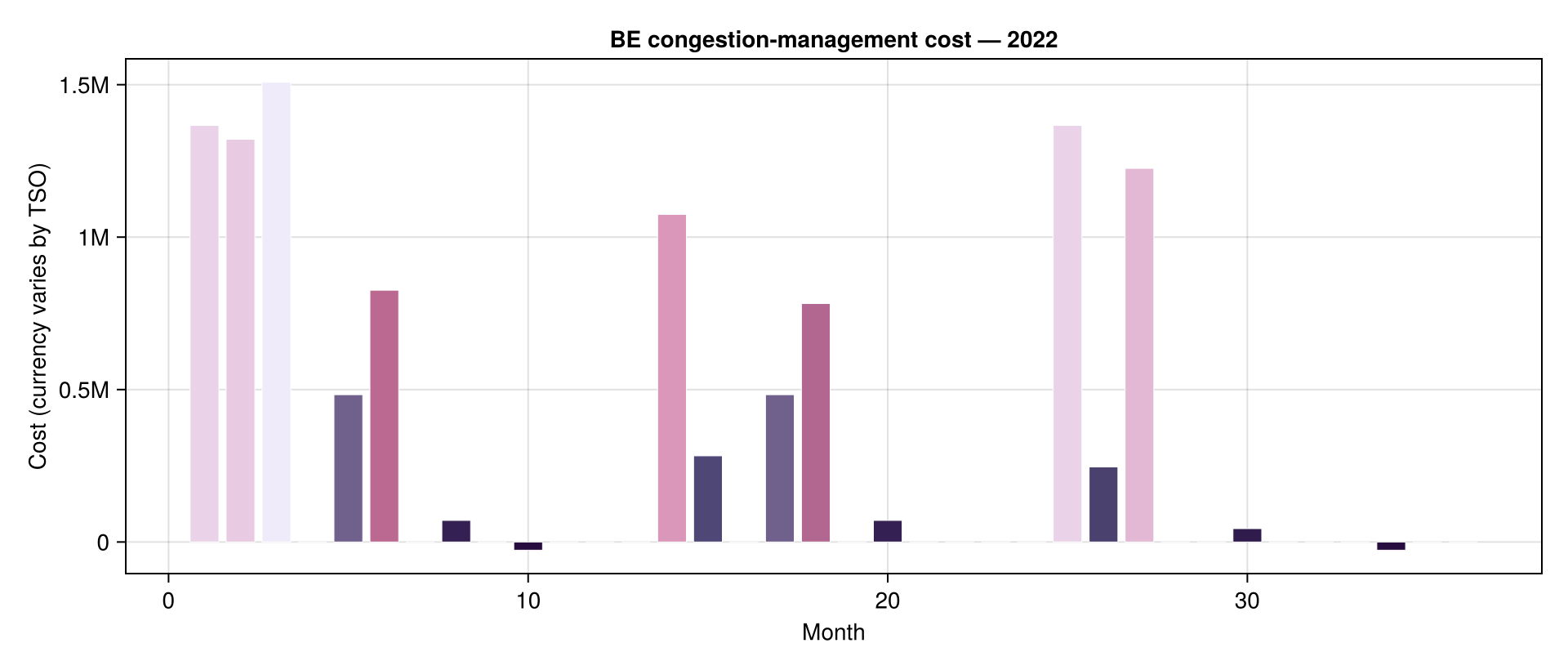

Redispatch volumes — three lenses

The three redispatch/countertrade endpoints have different time bases and zones; we stack them in a small-multiple to highlight the shape of each.

fig2 = Figure(size = (960, 540))

ax1 = Axis(fig2[1, 1];
    title = "Redispatching internal — NL, Nov 2023",
    ylabel = "MW")
isempty(redispatch_internal.value) ||
    barplot!(ax1, 1:length(redispatch_internal), redispatch_internal.value;
        color = :steelblue, strokewidth = 0.4, strokecolor = :white)

ax2 = Axis(fig2[2, 1];
    title = "Redispatching cross-border — FR ← AT, Nov 2023",
    ylabel = "MW")
isempty(redispatch_cross.value) ||
    barplot!(ax2, 1:length(redispatch_cross), redispatch_cross.value;
        color = :firebrick, strokewidth = 0.4, strokecolor = :white)

ax3 = Axis(fig2[3, 1];
    title = "Countertrading — FR ↔ ES, 13 Sep 2023",
    ylabel = "MW", xlabel = "Interval index")
isempty(counter.value) ||
    barplot!(ax3, 1:length(counter), counter.value;
        color = :seagreen, strokewidth = 0.4, strokecolor = :white)

linkxaxes!(ax1, ax2, ax3)
fig2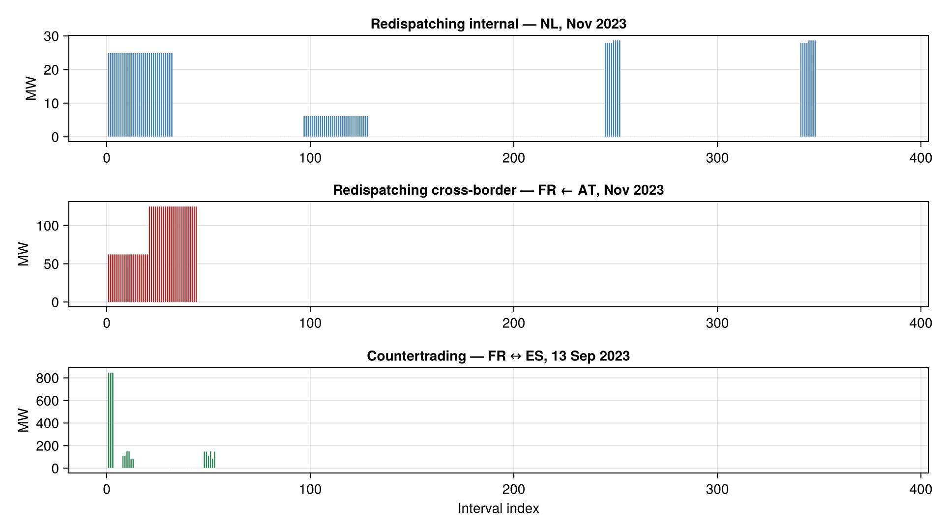

Sanity numbers

(
    annual_cost     = round(Int, sum(costs.value)),
    mean_monthly    = round(Int, mean(costs.value)),
    peak_month_cost = round(Int, maximum(costs.value)),
    nl_redispatch_total_mwh   = round(Int, sum(redispatch_internal.value)),
    fr_es_counter_total_mwh   = round(Int, sum(counter.value)),
)

(annual_cost = 11096637, mean_monthly = 308240, peak_month_cost = 1508142, nl_redispatch_total_mwh = 1454, fr_es_counter_total_mwh = 4034)

Where to next

• commercial_schedules and commercial_schedules_net_positions (Transmission 12.1.F) for what the market originally cleared — pair with the physical flows from cross_border_physical_flows to spot how much of the schedule the TSO had to actually re-route.

• forecasted_transfer_capacities (Transmission 11.1.A) for the NTC view ahead of time.

• current_balancing_state for the real-time view of how successfully the TSO closed the gap (see the PT1M balancing-state tutorial).