Tutorial: cross-border physical flows on the NL ↔ DE link
Realised flows on a single interconnector come from Transmission 12.1.G — wrapped here as cross_border_physical_flows. This tutorial pulls a full week (2024-09-02 → 2024-09-09) for the Netherlands ↔ Germany/Lux border and plots a signed time-series: positive when NL imports, negative when NL exports.
A small but important quirk: ENTSO-E reports each direction in its own document. To get the net flow you query both directions and subtract. Cassettes for both directions live alongside the tutorial.
Setup
using ENTSOE
using CairoMakie
using Dates

CairoMakie.activate!(type = "png")

include(joinpath(pkgdir(ENTSOE), "test", "_brokenrecord_helpers.jl"))
const BR = _load_brokenrecord()
client = ENTSOEClient("PLAYBACK")
Argument ordering
The wrapper takes (client, in_area, out_area, ...):
in_area— receiving zoneout_area— sending zone
Flows are reported positive when energy actually crosses into in_area. So the first call returns DE→NL flow (positive numbers when DE exports into NL):
de_to_nl = BR.playback("tut_flows_DE_to_NL_week.yml") do
    cross_border_physical_flows(
        client, EIC.NL, EIC.DE_LU,
        DateTime("2024-09-01T22:00"),
        DateTime("2024-09-08T22:00"))
end
length(de_to_nl), de_to_nl[1]
(672, (time = Dates.DateTime("2024-09-01T22:00:00"), value = 1269.56))…and the second the opposite direction (positive when NL exports into DE):
nl_to_de = BR.playback("tut_flows_NL_to_DE_week.yml") do
    cross_border_physical_flows(
        client, EIC.DE_LU, EIC.NL,
        DateTime("2024-09-01T22:00"),
        DateTime("2024-09-08T22:00"))
end
nl_to_de[1]
(time = Dates.DateTime("2024-09-01T22:00:00"), value = 0.0)Net flow
ENTSO-E publishes the two directions as separate (always-positive) series, hourly. Subtract them to get a signed net flow. The two direction-series sometimes carry slightly different first/last timestamps (DST shifts, missing hours), so we trim to the shared prefix length before subtracting. Column access on the StructVector makes this a one-liner:
n = min(length(de_to_nl), length(nl_to_de))
net = de_to_nl.value[1:n] .- nl_to_de.value[1:n]   # positive = NL importing
extrema(net)
(-3699.48, 2422.16)Plotting
fig = Figure(size = (900, 380))
ax = Axis(fig[1, 1];
    xlabel = "UTC time",
    ylabel = "MW (positive = NL importing)",
    title  = "NL ↔ DE physical flow — week of 2024-09-02",
)
band!(ax, 1:length(net), zero(net), net;
    color = (ifelse.(net .>= 0, :seagreen, :firebrick)))
lines!(ax, 1:length(net), net; color = :black, linewidth = 0.6)
hlines!(ax, [0]; color = :gray70, linewidth = 0.6)
ax.xticks = (
    1:24:length(net),
    [Dates.format(de_to_nl.time[i], "E dd") for i in 1:24:length(net)],
)
fig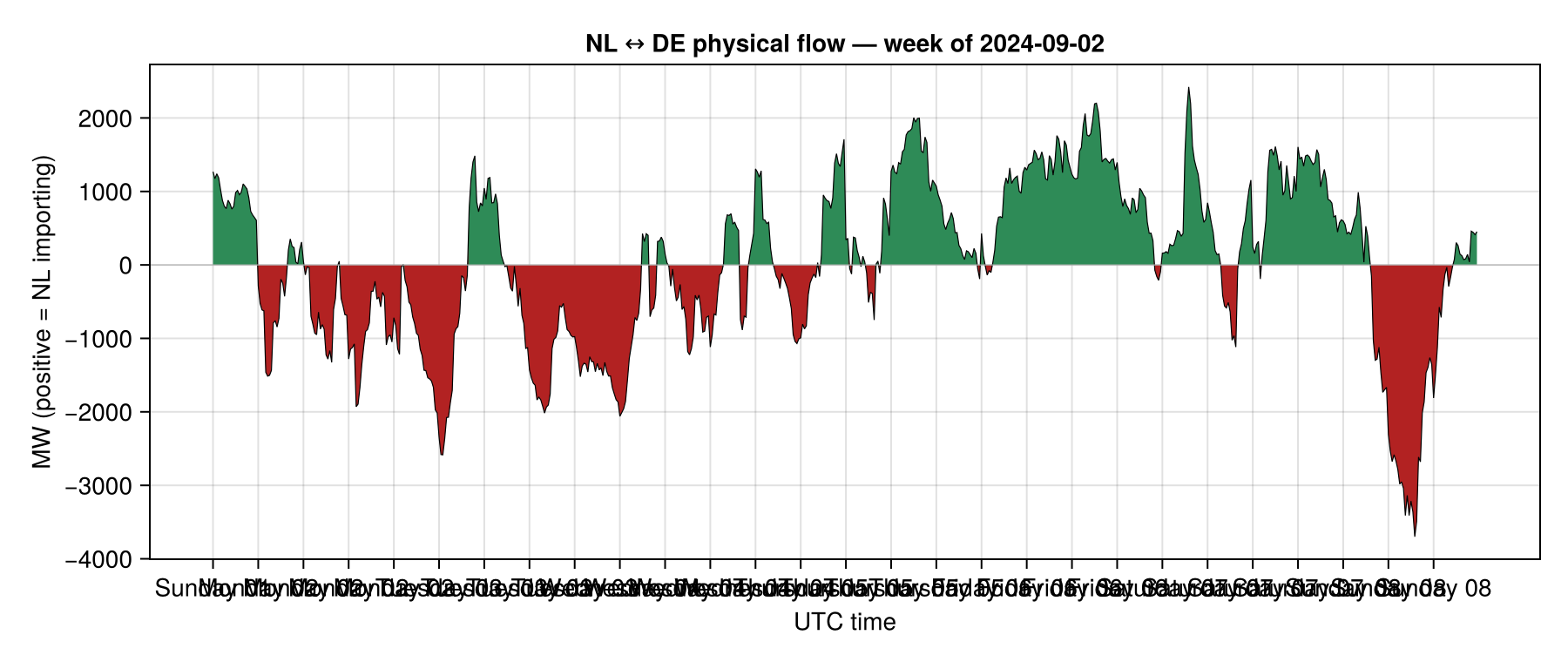
The visible pattern:
NL imports overnight (green), when its dispatchable fleet is scaled back and DE wind is plentiful.
NL exports during midday peaks (red), driven by Dutch solar generation when DE prices are high enough to pull power across the interconnector.
The trace mostly stays well inside the published NTC limits for the NL ↔ DE link (≈ 5 GW typical), which means nothing in our window was congested.
Aggregations
Because de_to_nl.value and nl_to_de.value are plain Vector{Float64}s, totalising the week's gross flow is one line:
hours_per_pt = 1.0  # 12.1.G is hourly resolution
import_gwh = sum(max.(net, 0)) * hours_per_pt / 1_000
export_gwh = sum(min.(net, 0)) * hours_per_pt / 1_000
(net_flow_gwh = round(import_gwh + export_gwh; digits = 2),
 imports_gwh  = round(import_gwh;  digits = 2),
 exports_gwh  = round(export_gwh;  digits = 2))
(net_flow_gwh = 10.64, imports_gwh = 318.45, exports_gwh = -307.81)Daily roll-up
Sum each day's signed flow into a single bar — easier to compare days at a glance than the hourly trace:
hours_per_day = 24
daily_gwh = [sum(@view net[(d - 1) * hours_per_day + 1:d * hours_per_day]) / 1_000
             for d in 1:(length(net) ÷ hours_per_day)]
day_labels = [Dates.format(de_to_nl.time[(d - 1) * hours_per_day + 1], "E dd")
              for d in eachindex(daily_gwh)]

fig2 = Figure(size = (760, 320))
ax = Axis(fig2[1, 1];
    xlabel = "Day",
    ylabel = "Net GWh (positive = NL imports)",
    title  = "NL ↔ DE-LU — daily net flow, week of 2024-09-02",
    xticks = (1:length(daily_gwh), day_labels),
)
hlines!(ax, [0]; color = :gray70, linewidth = 0.5)
barplot!(ax, 1:length(daily_gwh), daily_gwh;
    color = [v >= 0 ? :seagreen : :firebrick for v in daily_gwh],
    strokewidth = 0.5, strokecolor = :white)
fig2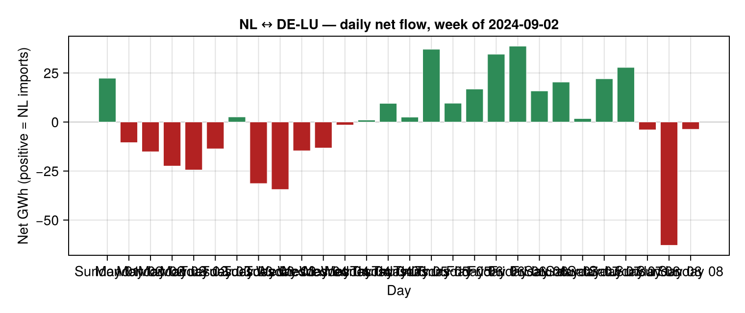
Where to next
For commercial (scheduled) cross-border allocations rather than realised physical flows, the relevant generated function is
transmission111_a_explicit_allocations(no convenience wrapper yet — call viaentsoe_apis(client).transmission).For multi-zone scans, write a loop over EIC pairs and aggregate the results. Ranges longer than ENTSO-E's per-call period limit are split into windows automatically — see the multi-year tutorial.