Tutorial: cross-border flow map of Europe

The two earlier map tutorials colour countries. Cross-border electricity, though, flows between bidding zones, and several countries are split into many — Norway has five, Sweden four, Denmark and Italy several each. This tutorial draws the real bidding-zone polygons and overlays every interconnector in the package's NEIGHBOURS graph as an arrow whose direction is the net exporter → importer and whose width and colour encode the transferred volume over a chosen time period.

The data layer is cross_border_physical_flows (Transmission 12.1.G, documentType=A11), pulled once per border in both directions and integrated from MW into energy (GWh) over the period. As with the price heat-map, the flows were pre-aggregated into a small JSON fixture committed at docs/src/assets/cross_border_flows_2025.json so the docs build stays offline; the recorder is scripts/record_flow_map.jl. We record one representative winter week (13–20 January 2025) — enough to show the structural picture without downloading a year of quarter-hour flows. Widen the period in the recorder and re-run for a longer window.

Bidding-zone polygons — credit

The zone shapes in docs/src/assets/bidding_zones/*.geojson are not original to ENTSOE.jl. They are vendored, unmodified and with gratitude, from the MIT-licensed entsoe-py package by EnergieID cvba-so and contributors. Their upstream sources (Natural Earth, NVE, redrawn Sweden, aggregated Italy) and the full attribution live in docs/src/assets/bidding_zones/ATTRIBUTION.md.

Setup

julia

using ENTSOE
using GeoMakie, CairoMakie
using GeoMakie: NaturalEarth
using GeoInterface
using GeoJSON
using Polylabel
using Proj                       # enables GeometryOps' Proj-backed extension
import GeometryOps as GO
using JSON

# Static map — CairoMakie's PNG output is all we need.
CairoMakie.activate!(type = "png")

The flow fixture

Each entry is one undirected border {a, b}, carrying the net energy a → b in GWh over the period (positive means a was, on balance, exporting to b), the gross energy each way, and the geojson zone stems a_zone / b_zone (or nothing for zones we have no polygon for — GB and Ireland, which are recorded but not drawn).

julia

const FIXTURE = joinpath(pkgdir(ENTSOE), "docs", "src", "assets",
                         "cross_border_flows_2025.json")
flows = JSON.parsefile(FIXTURE)
(period = flows["period_label"], n_borders = length(flows["borders"]))

(period = "2025-01-13 – 2025-01-20", n_borders = 49)

net_gwh just reads the signed a → b net energy for a border:

julia

net_gwh(border) = Float64(border["net_a_to_b_gwh"])

# Sweden (SE4) ↔ Germany over the week:
se4de = only(filter(flows["borders"]) do b
    Set((b["a_label"], b["b_label"])) == Set(("SE4", "DE-LU"))
end)
(border = "$(se4de["a_label"]) → $(se4de["b_label"])",
 net_gwh = round(net_gwh(se4de); digits = 1),
 gross_each_way_gwh = round.((se4de["gross_a_to_b_gwh"],
                             se4de["gross_b_to_a_gwh"]); digits = 1))

(border = "SE4 → DE-LU", net_gwh = 99.6, gross_each_way_gwh = (99.6, 0.0))

Zone polygons and projection-aware centroids

We draw every bidding zone we have a polygon for as the backdrop (skipping the pre-2021 _2020 duplicates so each zone appears once), and place each zone's label / arrow anchor with the same trick the sibling map tutorials use: take the largest sub-polygon by geodesic area (the mainland), reproject it into our Lambert Conformal Conic CRS, run Polylabel there, and reproject the pole of inaccessibility back to (lon, lat). Arrows are only drawn for borders whose both ends have a polygon.

julia

const PROJ_STR = "+proj=lcc +lat_1=35 +lat_2=65 +lat_0=50 +lon_0=10"
const WGS84    = "+proj=longlat +datum=WGS84"
const GEO_DIR  = joinpath(pkgdir(ENTSOE), "docs", "src", "assets", "bidding_zones")

load_zone(stem) = GeoJSON.read(read(joinpath(GEO_DIR, "$(stem).geojson"), String))

function label_lonlat(geom)
    sub_polys = GeoInterface.geomtrait(geom) isa GeoInterface.MultiPolygonTrait ?
        collect(GeoInterface.getgeom(geom)) : [geom]
    main = argmax(sub -> GO.area(GO.Geodesic(), sub), sub_polys)
    pole = polylabel(GO.reproject(main, WGS84, PROJ_STR); rtol = 0.005)
    pt = GO.reproject(GeoInterface.Wrappers.Point(pole...), PROJ_STR, WGS84)
    return (GeoInterface.x(pt), GeoInterface.y(pt))
end

# Every bidding zone we have a polygon for, minus the pre-2021 `_2020`
# duplicates (IT_CNOR/CSUD/SUD) so each zone is drawn exactly once.
zone_stems = sort([replace(f, ".geojson" => "") for f in readdir(GEO_DIR)
                   if endswith(f, ".geojson") && !endswith(f, "_2020.geojson")])

geom_by_zone   = Dict(z => GeoInterface.geometry(load_zone(z)[1]) for z in zone_stems)
center_by_zone = Dict(z => label_lonlat(g) for (z, g) in geom_by_zone)
length(zone_stems)

For geographic context we also draw every other European country — the ones we don't model as bidding zones (UK, the western Balkans, …) — from Natural Earth's Admin-0 set, in a lighter shade. And we highlight the Core Capacity Calculation Region (Core CCR), the zones that clear day-ahead capacity together under flow-based market coupling. Ireland belongs to Core too, via the Celtic Interconnector (IE↔FR), but we hold no bidding-zone polygon for it, so it's coloured from its Natural Earth country outline instead:

julia

countries_fc = NaturalEarth.naturalearth("admin_0_countries", 50)

function _country_iso2(feature)
    p = feature.properties
    for key in (:ISO_A2_EH, :ISO_A2)
        v = get(p, key, nothing)
        v === nothing && continue
        v isa AbstractString && v != "-99" && return String(v)
    end
    return ""
end

const CORE_CCR = Set(["AT", "BE", "HR", "CZ", "FR", "DE_LU", "HU", "NL",
                      "PL", "RO", "SK", "SI"])

# Core members we hold no bidding-zone polygon for, coloured via their
# Natural Earth outline instead. Ireland is in Core through the Celtic
# Interconnector (IE↔FR border) — see ENTSO-E's CCR Regions map.
const CORE_BACKDROP_ISO2 = Set(["IE"])

const OTHER_COUNTRY = RGBAf(0.93, 0.93, 0.93, 1)     # non-modelled: very light grey
const OTHER_ZONE    = RGBAf(0.86, 0.95, 0.86, 1)     # modelled non-Core: very light green
const CORE_COLOR    = RGBAf(0.78, 0.88, 0.97, 0.7)   # Core CCR: very light blue

Placing every endpoint, including the polygon-less ones

Each interconnector is drawn as a plain line between its two zones' centroids. Most endpoints are geojson zones, but some borders touch zones we have no polygon for — Great Britain and Ireland. We still have their flow data (the neighbouring side publishes it), so we position them from their Natural Earth country centroid and they draw normally. This is what adds the GB interconnectors (to FR, BE, NL, NO2, DK1, IE).

julia

const EXTRA_ISO2 = Dict("10YGB----------A" => "GB", "10Y1001A1001A59C" => "IE")

function country_center(iso2)
    for feat in countries_fc
        _country_iso2(feat) == iso2 && return label_lonlat(feat.geometry)
    end
    error("no Natural Earth country for $iso2")
end
extra_center_by_iso2 = Dict(v => country_center(v) for v in values(EXTRA_ISO2))

# Position of every placeable endpoint, keyed by EIC: a geojson centroid,
# else a Natural Earth country centroid for GB / IE.
pos_by_eic = Dict{String, Tuple{Float64, Float64}}()
for b in flows["borders"],
        (eic, zone) in ((b["a_eic"], b["a_zone"]), (b["b_eic"], b["b_zone"]))
    haskey(pos_by_eic, eic) && continue
    if zone !== nothing
        pos_by_eic[eic] = center_by_zone[zone]
    elseif haskey(EXTRA_ISO2, eic)
        pos_by_eic[eic] = extra_center_by_iso2[EXTRA_ISO2[eic]]
    end
end

struct Link
    a::String; b::String   # EICs
    mag::Float64           # |net| GWh over the period
end

function build_links(borders)
    out = Link[]
    for b in borders
        (haskey(pos_by_eic, b["a_eic"]) && haskey(pos_by_eic, b["b_eic"])) || continue
        v = abs(net_gwh(b))
        iszero(v) && continue
        push!(out, Link(b["a_eic"], b["b_eic"], v))
    end
    return sort(out; by = l -> l.mag)   # thin drawn first, thick on top
end

links = build_links(flows["borders"])
maxmag = maximum(l -> l.mag, links)
(n_links = length(links), max_gwh = round(maxmag; digits = 1))

(n_links = 49, max_gwh = 474.0)

The map

We stack three fill layers — non-modelled countries, modelled zones, Core CCR highlighted — draw the interconnectors on top as plain black lines whose thickness encodes the net volume, and pair a line-thickness key with a category legend for the fills.

julia

# Line width encodes volume (∝ √GWh); colour is a constant black.
lw(mag) = 0.8 + 5.0 * sqrt(mag / maxmag)

function draw_flow_map(links, maxmag; title)
    fig = Figure(size = (820, 620))
    ax  = GeoAxis(fig[1, 1];
        dest = PROJ_STR,
        limits = ((-12, 34), (35, 71)),
        title = title,
        xgridvisible = false, ygridvisible = false,
        xticksvisible = false, yticksvisible = false,
        xticklabelsvisible = false, yticklabelsvisible = false,
    )

    # Layer 1: every other European country as light context, with any
    # polygon-less Core member (Ireland) highlighted like the Core zones.
    for feat in countries_fc
        core = _country_iso2(feat) in CORE_BACKDROP_ISO2
        poly!(ax, feat.geometry; color = core ? CORE_COLOR : OTHER_COUNTRY,
            strokecolor = :white, strokewidth = core ? 0.5 : 0.4)
    end
    # Layer 2: modelled bidding zones, with Core CCR highlighted.
    for (z, g) in geom_by_zone
        poly!(ax, g; color = z in CORE_CCR ? CORE_COLOR : OTHER_ZONE,
            strokecolor = :white, strokewidth = 0.5)
    end

    # Interconnectors: plain black lines, full centroid-to-centroid,
    # thickness ∝ volume. No arrowheads, so undirected.
    for l in links
        s, d = pos_by_eic[l.a], pos_by_eic[l.b]
        lines!(ax, [s[1], d[1]], [s[2], d[2]]; color = :black, linewidth = lw(l.mag))
    end

    # Zone codes (underscores stripped), plus GB / IE from country centroids.
    # Each label gets an opaque white pill behind it (masking the lines it
    # crosses) so the black text stays readable. Pills first, then text.
    labels = [(c, replace(z, "_" => "")) for (z, c) in center_by_zone]
    append!(labels, [(extra_center_by_iso2[i], i) for i in ("GB", "IE")])
    for (c, s) in labels
        scatter!(ax, [c[1]], [c[2]]; marker = :circle,
            markersize = Vec2f(7.5 * length(s) + 16, 22), color = (:white, 0.85),
            glowwidth = 6, glowcolor = (:white, 0.55))
    end
    for (c, s) in labels
        text!(ax, c...; text = s, align = (:center, :center),
            fontsize = 11, color = :black, font = :bold)
    end

    # Bottom legends, grouped together and centred: area fills on the
    # left, the line-thickness (volume) key on the right.
    area_elems = [
        PolyElement(color = CORE_COLOR, strokecolor = :white, strokewidth = 1),
        PolyElement(color = OTHER_ZONE, strokecolor = :white, strokewidth = 1),
    ]
    lvls = round.(Int, [0.2, 0.5, 0.9] .* maxmag ./ 50) .* 50
    lw_elems = [LineElement(color = :black, linewidth = lw(v)) for v in lvls]

    legrid = GridLayout(fig[2, 1]; tellwidth = false, halign = :center)
    Legend(legrid[1, 1], area_elems, ["Core CCR", "Other"];
        orientation = :horizontal, framevisible = true, nbanks = 1,
        tellheight = true, tellwidth = true, patchsize = (18, 12))
    Legend(legrid[1, 2], lw_elems, ["$(v) GWh" for v in lvls];
        orientation = :horizontal, framevisible = true, nbanks = 1,
        tellheight = true, tellwidth = true, patchsize = (36, 14))
    colgap!(legrid, 14)
    rowgap!(fig.layout, 4)
    return fig
end

draw_flow_map(links, maxmag;
    title = "Net cross-border electricity flows, 13–20 Jan 2025 (GWh)")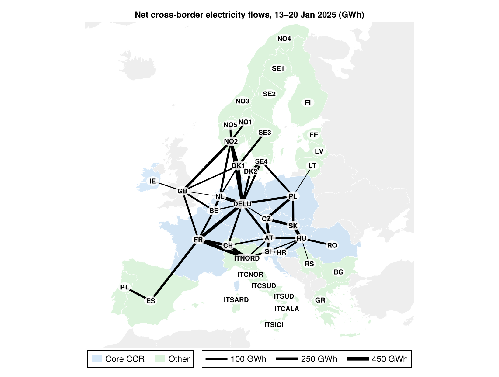

The lines trace Europe's interconnector backbone over the week: the thick strands out of France into Switzerland and Italy, the Nordic links feeding south, Germany's dense hub, and — now that GB and IE are placed from their country outlines — the North Sea and Channel cables (GB↔NO2, GB↔FR, GB↔NL, GB↔BE, GB↔IE). Thickness is the net transferred energy; thin lines are low-volume or near-balanced links.

Picking a different period

"A given time period" lives entirely in the recorder: change PERIOD_START / PERIOD_END in scripts/record_flow_map.jl, re-run it with a token, and the next docs build redraws the same network for the new window. Everything downstream — the lines, their widths, the thickness key — keys off net_a_to_b_gwh, so nothing here changes.

Extending it

More borders: add the pair to NEIGHBOURS and re-run scripts/record_flow_map.jl with a token — the map keys entirely off the fixture and the EIC → zone crosswalk in that script.
More zones: drop the matching *.geojson into docs/src/assets/bidding_zones/ (keeping the entsoe-py attribution) and add its stem to the crosswalk.

Where to next

A single border as a time series rather than an annual total: NL ↔ DE cross-border flows.
The same GeoAxis recipe coloured by price or renewables share: 2025 price heat-map and renewables-share map.

Tutorial: cross-border flow map of Europe ​

Setup ​

The flow fixture ​

Zone polygons and projection-aware centroids ​

Placing every endpoint, including the polygon-less ones ​

The map ​

Picking a different period ​

Extending it ​

Where to next ​

Tutorial: cross-border flow map of Europe

Setup

The flow fixture

Zone polygons and projection-aware centroids

Placing every endpoint, including the polygon-less ones

The map

Picking a different period

Extending it

Where to next