Tutorial: a day in the Dutch generation mix

Where did the electrons in NL come from on 2 September 2024? This page pulls one document from the Generation 16.1.B/C endpoint (actual_generation_per_production_type) and turns its TimeSeries-per-production-type structure into a stacked-area plot.

Like the rest of the tutorial set, the HTTP traffic is served from a cassette under test/cassettes/tut_gen_mix_NL_2024_09_02.yml, recorded once with a real token (see scripts/record_tutorial_cassettes.jl).

Setup

using ENTSOE
using CairoMakie
using Dates

CairoMakie.activate!(type = "png")

include(joinpath(pkgdir(ENTSOE), "test", "_brokenrecord_helpers.jl"))
const BR = _load_brokenrecord()
client = ENTSOEClient("PLAYBACK")

Fetching one day, every technology

actual_generation_per_production_type returns one TimeSeries per PSR_LABELS (Solar, Wind Onshore, Nuclear, Fossil Gas, …); each TimeSeries carries quarter-hour points. The wrapper parses every row and tags it with its psr_type code.

gen = BR.playback("tut_gen_mix_NL_2024_09_02.yml") do
    actual_generation_per_production_type(
        client, EIC.NL,
        DateTime("2024-09-01T22:00"),    # 2024-09-02 00:00 CET
        DateTime("2024-09-02T22:00"))
end
length(gen), gen[1]

(1920, (time = Dates.DateTime("2024-09-01T22:00:00"), psr_type = "B01", value = 0.0))

The result is a Tables.jl-compatible StructVector. Let's group it into one column per technology — column access (gen.psr_type, gen.value, gen.time) is zero-allocation, so the pivot is cheap:

function pivot_by_psr(rows)
    psr_codes = unique(rows.psr_type)
    times = sort!(unique(rows.time))
    out = Dict{String, Vector{Float64}}()
    for code in psr_codes
        col = zeros(Float64, length(times))
        time_idx = Dict(t => i for (i, t) in enumerate(times))
        for r in rows[rows.psr_type .== code]
            col[time_idx[r.time]] = r.value
        end
        out[code] = col
    end
    return (times = times, mix = out)
end

p = pivot_by_psr(gen)
sort(collect(keys(p.mix)))

10-element Vector{String}:
 "B01"
 "B04"
 "B05"
 "B11"
 "B14"
 "B16"
 "B17"
 "B18"
 "B19"
 "B20"

Stacked-area plot

Order matters for stacked plots — we want a stable order, dispatchable sources at the bottom, intermittent renewables on top. Pick a small palette covering NL's actual fleet (codes that don't appear in the fixture get skipped):

const STACK_ORDER = [
    ("B14", "Nuclear",       :gold),
    ("B05", "Hard coal",     :gray35),
    ("B04", "Fossil gas",    :firebrick),
    ("B17", "Waste",         :saddlebrown),
    ("B01", "Biomass",       :darkgreen),
    ("B11", "Hydro RoR",     :royalblue),
    ("B19", "Wind onshore",  :seagreen),
    ("B18", "Wind offshore", :steelblue),
    ("B16", "Solar",         :orange),
]

stacked = filter(t -> haskey(p.mix, t[1]), STACK_ORDER)
fig = Figure(size = (900, 460))
ax = Axis(fig[1, 1];
    xlabel = "UTC time",
    ylabel = "MW",
    title  = "NL generation by production type — 2024-09-02 (UTC)",
    xticks = (1:6:length(p.times),
              [Dates.format(p.times[i], "HH:MM") for i in 1:6:length(p.times)]),
)

cum = zeros(length(p.times))
for (code, label, color) in stacked
    series = p.mix[code]
    band!(ax, 1:length(p.times), cum, cum .+ series;
        color = color, label = "$(label) ($code)")
    cum .+= series
end
axislegend(ax; position = :rt, framevisible = false, labelsize = 10)
fig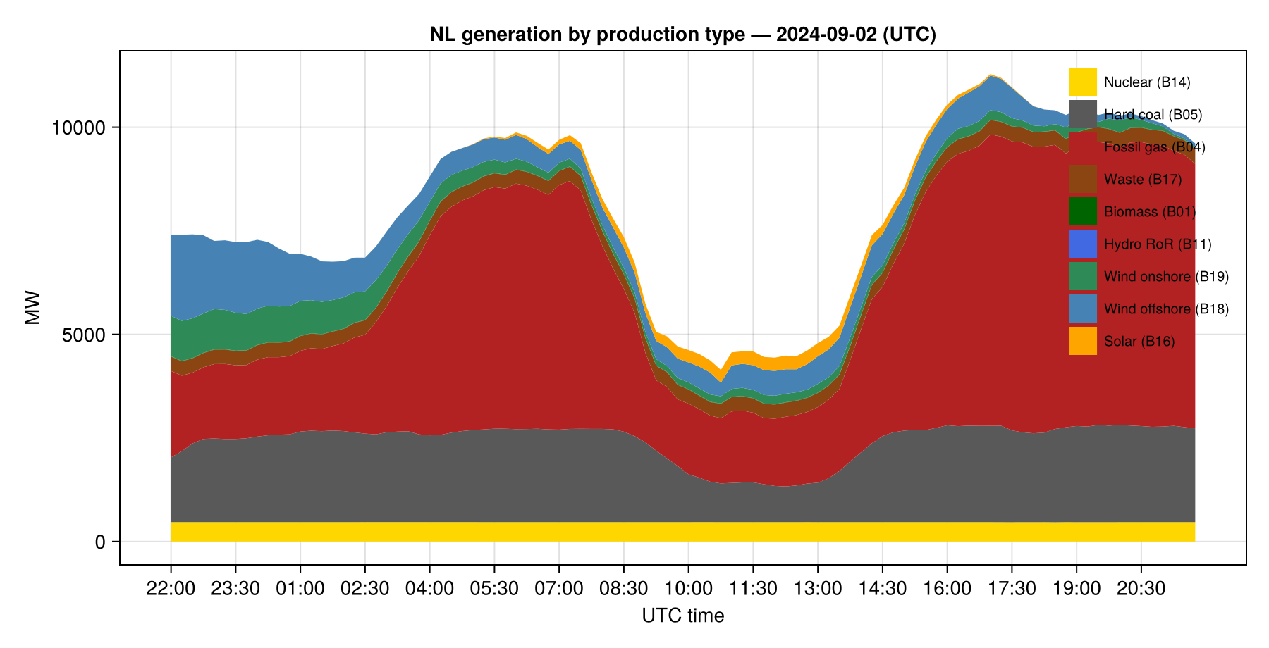

A few things to read off the plot:

• Solar ramps in around 06:00 UTC (08:00 CET) and peaks near noon; together with wind it covers a big chunk of the daytime load.

• Fossil gas does the residual-balancing — it visibly fills the evening shoulder once solar drops.

• Nuclear sits flat at the bottom because Borssele runs as baseload.

Aggregations on the column views

Because gen is a StructVector, day-totals fall out as column operations — no per-row indirection:

total_mwh = sum(gen.value) * 0.25   # quarter-hour points → MWh
solar_mwh = sum(gen.value[gen.psr_type .== PsrType.SOLAR]) * 0.25
wind_mwh  = sum(gen.value[in.(gen.psr_type, Ref(PsrGroup.WIND))]) * 0.25
(total_mwh = round(Int, total_mwh),
 solar_mwh = round(Int, solar_mwh),
 wind_mwh  = round(Int, wind_mwh),
 vre_share = round(100 * (solar_mwh + wind_mwh) / total_mwh; digits = 1))

(total_mwh = 315716, solar_mwh = 2471, wind_mwh = 25395, vre_share = 8.8)

Day-total bar chart

Same data, different lens — the share of each technology in the day's total energy rather than its instantaneous power:

day_totals = [
    (label = lbl, code = code, color = color,
     mwh   = sum(gen.value[gen.psr_type .== code]) * 0.25)
    for (code, lbl, color) in stacked
]

fig2 = Figure(size = (820, 380))
ax = Axis(fig2[1, 1];
    xlabel = "MWh",
    title  = "NL — energy by production type, 2024-09-02",
    yticks = (1:length(day_totals), [d.label for d in day_totals]),
)
barplot!(ax, 1:length(day_totals), [d.mwh for d in day_totals];
    direction = :x,
    color = [d.color for d in day_totals],
    strokewidth = 0.4, strokecolor = :white)
fig2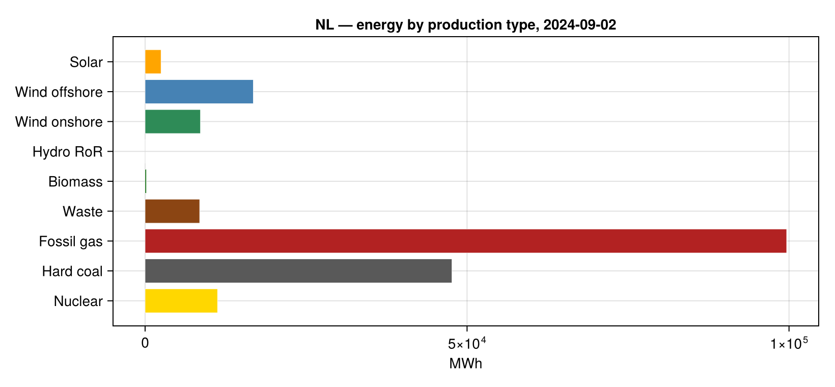

Where to next

• The same wrapper takes a psr_type= kwarg to pull a single technology server-side — handy if you only need solar: actual_generation_per_production_type(client, EIC.NL, t1, t2; psr_type = PsrType.SOLAR).

• Forecasts of just wind+solar (one document) are exposed via wind_solar_forecast.

• For the installed (year-ahead declared) capacity by PSR type, see installed_capacity_per_production_type used in the first tutorial.