Tutorial: five years of NL day-ahead prices

ENTSO-E caps most time-series endpoints at one year per request. You don't have to think about that limit: every time-series wrapper splits long ranges automatically. Hand a multi-year window to day_ahead_prices directly and the wrapper chunks the period internally, calls the endpoint once per chunk, skips empty windows, and concatenates the results into a single StructVector.

This tutorial walks 2020 through 2024 of Dutch day-ahead prices — five yearly cassettes pre-recorded under test/cassettes/tut_prices_NL_<year>.yml and replayed offline.

Setup

using ENTSOE
using CairoMakie
using Statistics: mean, median, quantile
using Dates

CairoMakie.activate!(type = "png")

include(joinpath(pkgdir(ENTSOE), "test", "_brokenrecord_helpers.jl"))
const BR = _load_brokenrecord()
client = ENTSOEClient("PLAYBACK")

One call, five chunks

Just call the wrapper over the whole range — the period-arithmetic happens inside it:

prices = BR.playback("tut_prices_NL_2020_2024.yml") do
    day_ahead_prices(
        client, EIC.NL,
        DateTime("2019-12-31T23:00"),
        DateTime("2024-12-31T23:00"),
    )
end
length(prices), prices[1], prices[end]

(43848, (time = Dates.DateTime("2019-12-31T23:00:00"), value = 41.88), (time = Dates.DateTime("2024-12-31T22:00:00"), value = 0.52))

Internally, the single call expanded into five day_ahead_prices(...) — one per yearly window — and vcat'd the resulting StructVectors. The chunk size comes from a window keyword whose default is Year(1) for this endpoint; pass window = Month(1) (or anything coarser/finer) to override it, e.g. to stay under a rate limit. Each chunk is hourly (8 760-ish points), so the whole window lands at ~44 k rows. BrokenRecord captured all five HTTP responses in one cassette during recording; the playback above replays them in the same order.

Yearly distributions

With five years of hourly prices in one StructVector, the column view (prices.value) is a plain Vector{Float64} and we can pivot on year for a box plot. Years have different lengths (DST + the odd incomplete chunk), so we materialise a long-form (year, value) pair list rather than an equal-shape matrix:

years = year.(prices.time)

xs = Int[]
ys = Float64[]
for y in 2020:2024
    mask = years .== y
    append!(ys, prices.value[mask])
    append!(xs, fill(y, count(mask)))
end

fig = Figure(size = (820, 460))
ax = Axis(fig[1, 1];
    xlabel = "Year",
    ylabel = "EUR / MWh",
    title  = "NL day-ahead prices, 2020-2024 (hourly)",
)
boxplot!(ax, xs, ys;
    width = 0.6, mediancolor = :white, color = :steelblue,
)
ax.xticks = (2020:2024, string.(2020:2024))
fig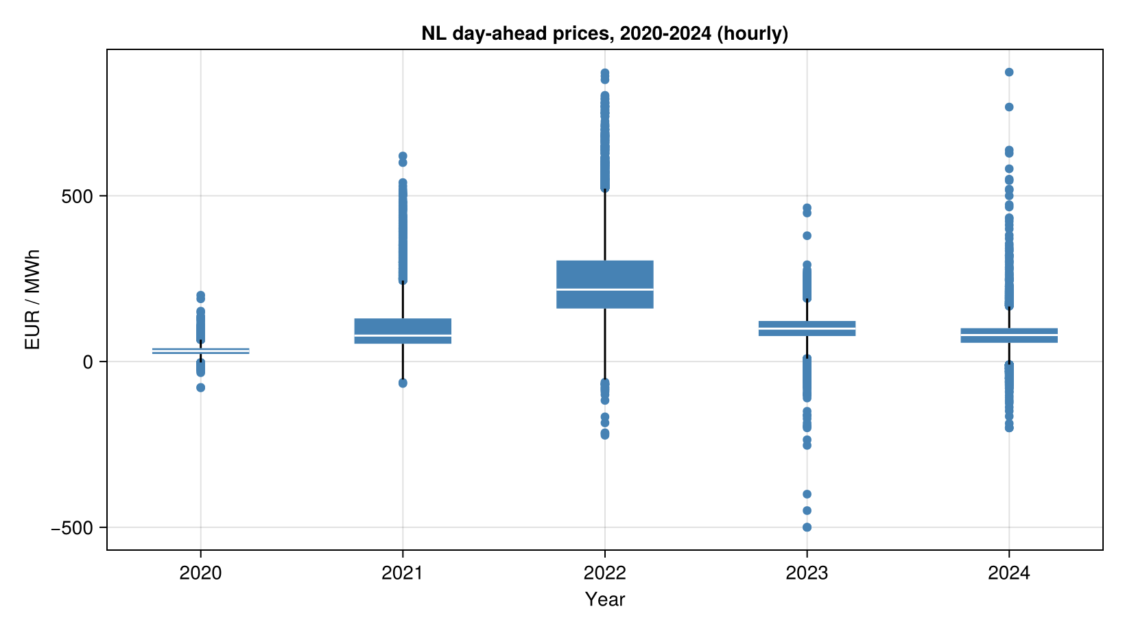

The picture matches the well-known story:

• 2020 — covid-quiet, very low prices (annual average around €30 / MWh).

• 2021–2022 — the gas crisis: 2021 ramps up, 2022 shows the highest medians by far, with a long upper tail.

• 2023–2024 — partial normalisation, but still well above the 2020 baseline.

Quick stats per year

StructVector columns are plain typed vectors — annual statistics are one-liners:

function summarise(year_prices)
    p = year_prices
    return (
        mean      = round(mean(p);            digits = 2),
        median    = round(median(p);          digits = 2),
        p95       = round(quantile(p, 0.95);  digits = 2),
        max       = round(maximum(p);         digits = 2),
        negative  = count(<(0), p),
    )
end

[(year = y, summarise(prices.value[years .== y])...) for y in 2020:2024]

5-element Vector{@NamedTuple{year::Int64, mean::Float64, median::Float64, p95::Float64, max::Float64, negative::Int64}}:
 (year = 2020, mean = 32.24, median = 31.67, p95 = 55.9, max = 200.04, negative = 97)
 (year = 2021, mean = 102.97, median = 78.31, p95 = 250.1, max = 620.0, negative = 70)
 (year = 2022, mean = 241.91, median = 217.0, p95 = 495.0, max = 871.0, negative = 86)
 (year = 2023, mean = 95.82, median = 99.22, p95 = 166.56, max = 463.77, negative = 315)
 (year = 2024, mean = 77.3, median = 80.0, p95 = 138.98, max = 872.96, negative = 458)

The negative column counts hours with a negative clearing price — a signal of oversupply (windy + sunny + low demand). 2024 has the most by far in this snapshot, which tracks NL's solar build-out.

Monthly mean trace

ym = [(year(t), month(t)) for t in prices.time]
unique_ym = sort!(unique(ym))
# `ym .== ym0` would broadcast over the 2-tuple `ym0`; wrap in `Ref` so
# each tuple is compared against the whole `ym0` as a single value.
monthly = [mean(prices.value[ym .== Ref(ym0)]) for ym0 in unique_ym]

fig2 = Figure(size = (900, 320))
ax2 = Axis(fig2[1, 1];
    xlabel = "",
    ylabel = "EUR / MWh",
    title  = "NL day-ahead price — monthly mean",
)
lines!(ax2, 1:length(monthly), monthly; color = :firebrick, linewidth = 1.6)
ax2.xticks = (
    [findfirst(==((y, 1)), unique_ym) for y in 2020:2024],
    string.(2020:2024),
)
fig2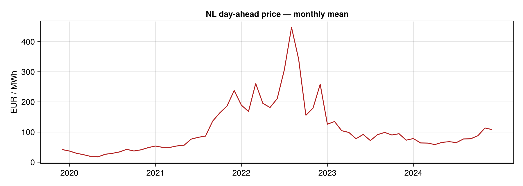

Where to next

• Automatic splitting works for every time-series wrapper — e.g. actual_total_load, cross_border_physical_flows, forecasts, generation per type. Each carries its own window default (Year(1) for most; Day(1) for the balancing-bid / activated-energy family, which ENTSO-E caps at one day). Override it with the window keyword when you want finer chunks.

• Empty chunks (ENTSOEAcknowledgement reason 999) are skipped automatically — so a 5-year request that spans some incomplete months still returns whatever is available. Only if every window is empty does the acknowledgement propagate.

• The response-format dispatch works across the split too: pass Raw() as a trailing positional arg and the per-window XML bodies come back concatenated with a <!-- next window --> sentinel between them.

• Want the chunk boundaries themselves? split_period is the exposed arithmetic primitive — give it (start, stop; window) and it returns the Vector{Tuple{DateTime,DateTime}} the wrappers use.