Tutorial: 1 440 PT1M samples of Hungary's area control error

The Balancing 1.2.3.A endpoint publishes the area-control-error trajectory at PT1M resolution — that's 1 440 samples per day. The wrapper is current_balancing_state; the parser is the familiar parse_timeseries, which knows the PT1M case is real (it was added when this endpoint started returning sub-quarter-hour data).

This page draws what 24 hours of minute-by-minute imbalance looks like in a real control area — the wiggle is meaningful, not noise.

Setup

using ENTSOE
using CairoMakie
using Dates
using Statistics: mean, median, quantile

CairoMakie.activate!(type = "png")

include(joinpath(pkgdir(ENTSOE), "test", "_brokenrecord_helpers.jl"))
const BR = _load_brokenrecord()
client = ENTSOEClient("PLAYBACK")

Fetch one day

BusinessType.AREA_CONTROL_ERROR (IEC 62325 code B33) is the difference between scheduled and actual cross-border exchange.

ace = BR.playback("tut_balancing_state_HU_2024.yml") do
    current_balancing_state(
        client, EIC.HU,
        DateTime("2024-05-29T22:00"), DateTime("2024-05-30T22:00");
        business_type = BusinessType.AREA_CONTROL_ERROR,
    )
end
length(ace), ace[1]

(1440, (time = Dates.DateTime("2024-05-29T22:00:00"), value = 4.07))

24 × 60 = 1 440 minute-resolution rows for one trading day.

The minute-by-minute wiggle

This is the signature plot — most ENTSO-E series are quarter-hourly, which smooths out the actual control dynamics. PT1M reveals them.

# X-tick positions every 2 hours (= every 120 PT1M samples) with HH:MM labels.
n = length(ace)
tick_idx = 1:120:n
tick_labels = [Dates.format(ace.time[i], "HH:MM") for i in tick_idx]

fig = Figure(size = (1100, 380))
ax = Axis(fig[1, 1];
    title  = "HU area control error — 30 May 2024, PT1M",
    xlabel = "UTC time",
    ylabel = "Imbalance (MW; +export / −import)",
    xticks = (tick_idx, tick_labels),
)
lines!(ax, 1:n, ace.value;
    color = :darkorange, linewidth = 0.8)
hlines!(ax, [0]; color = :black, linewidth = 0.6)
# Light ±1σ shaded band to give scale.
σ = round(quantile(abs.(ace.value), 0.68); digits = 0)
hspan!(ax, -σ, σ; color = (:darkorange, 0.06))
fig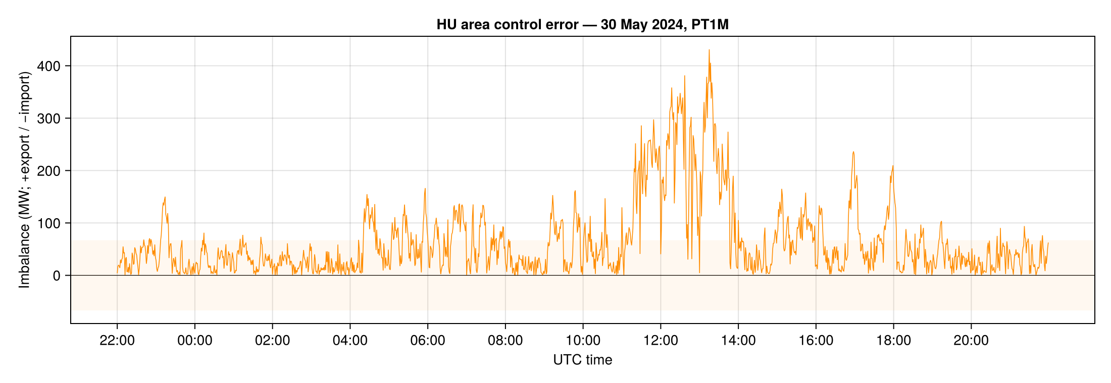

The trace oscillates around zero on a ~10-minute timescale — those are the secondary control loops (aFRR) working to restore the schedule.

Histogram of |imbalance|

fig2 = Figure(size = (640, 360))
ax = Axis(fig2[1, 1];
    title  = "HU |ACE| distribution — 1 440 minutes",
    xlabel = "|Imbalance| (MW)",
    ylabel = "Count",
)
hist!(ax, abs.(ace.value);
    bins = 30, color = :darkorange, strokewidth = 0.4, strokecolor = :white)
# Mark the 95th percentile as a vertical line.
p95 = quantile(abs.(ace.value), 0.95)
vlines!(ax, [p95]; color = :black, linestyle = :dash, linewidth = 1)
text!(ax, p95, 0; text = " 95th pct = $(round(Int, p95)) MW",
    align = (:left, :bottom), fontsize = 11, color = :black)
fig2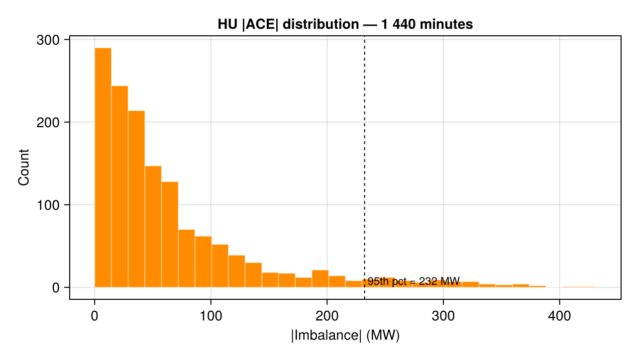

Quick-look stats

(
    samples              = length(ace),
    mean_signed_mw       = round(mean(ace.value); digits = 1),
    median_abs_mw        = round(median(abs.(ace.value)); digits = 1),
    max_abs_mw           = round(Int, maximum(abs.(ace.value))),
    minutes_within_50mw  = count(abs.(ace.value) .<= 50),
)

(samples = 1440, mean_signed_mw = 65.6, median_abs_mw = 41.1, max_abs_mw = 431, minutes_within_50mw = 821)

The system spent the bulk of the day inside ±50 MW — a tight band relative to the country's ~5 GW peak load.

A note on resolutions

The PT1M resolution caught us off guard once: earlier versions of parse_timeseries only handled PT15M/PT30M/PT60M and longer; querying HU's balancing state crashed with "unsupported ENTSO-E resolution PT1M". The fix added PT1M (plus PT5M/PT10M) to the supported set, and now unknown resolutions emit a one-shot @warn and skip the offending Period rather than crashing — so a future PT2M won't break your batch import.

Where to next

• aggregated_balancing_energy_bids for the actual aFRR bid prices the TSO was activating during these minutes.

• imbalance_prices and total_imbalance_volumes for the settlement view of what every minute of imbalance ended up costing — see the imbalance-market tutorial.