Tutorial: Bulgarian hydro reservoirs

Generation 16.1.D publishes the filled energy in a control area's hydro reservoirs and pumped-storage plants — one quantity per week, in MWh. The wrapper water_reservoirs_and_hydro_storage_plants returns a (time, value) StructVector; we plot a snapshot week here and combine it with the installed hydro capacity for context.

Setup

using ENTSOE
using CairoMakie
using Dates

CairoMakie.activate!(type = "png")

include(joinpath(pkgdir(ENTSOE), "test", "_brokenrecord_helpers.jl"))
const BR = _load_brokenrecord()
client = ENTSOEClient("PLAYBACK")

Fetch — one week, then compare to installed capacity

hydro = BR.playback("tut_hydro_BG_2023.yml") do
    water_reservoirs_and_hydro_storage_plants(
        client, EIC.BG,
        DateTime("2023-07-09T21:00"), DateTime("2023-07-16T21:00"),
    )
end
hydro

1-element StructArray(::Vector{Dates.DateTime}, ::Vector{Float64}) with eltype @NamedTuple{time::Dates.DateTime, value::Float64}:
 (time = Dates.DateTime("2023-07-09T21:00:00"), value = 1.90968774e6)

For broader context, pull the installed-capacity registry on the same control area and isolate the hydro PSR types:

PsrGroup bundles the three hydro PSR codes (B10 pumped storage, B11 run-of-river, B12 reservoir) into a single tuple — useful for client-side filtering of a fetched table:

# Reuse a smoke cassette so this works offline; it covers NL but the
# document shape is identical across zones.
caps = BR.playback("generation_141a_installed_capacity_NL.yml") do
    installed_capacity_per_production_type(
        client, EIC.NL,
        DateTime("2023-12-31T23:00"), DateTime("2024-12-31T23:00"),
    )
end
hydro_caps = caps[in.(caps.psr_type, Ref(PsrGroup.HYDRO))]
hydro_caps

3-element StructArray(::Vector{String}, ::Vector{Float64}) with eltype @NamedTuple{psr_type::String, capacity_mw::Float64}:
 (psr_type = "B10", capacity_mw = 0.0)
 (psr_type = "B11", capacity_mw = 38.0)
 (psr_type = "B12", capacity_mw = 0.0)

PsrGroup also exposes WIND, FOSSIL, RENEWABLE, STORAGE, and INFRASTRUCTURE for the same pattern. For a single-technology filter on the server, pass the scalar PsrType constant to the wrapper's psr_type kwarg — e.g. actual_generation_per_production_type(...; psr_type = PsrType.HYDRO_WATER_RESERVOIR).

Stored energy across the week

fig = Figure(size = (840, 360))
ax = Axis(fig[1, 1];
    title  = "BG hydro reservoir filling — week of 9 Jul 2023",
    xlabel = "Reading",
    ylabel = "Stored energy (MWh)",
    xticks = (1:length(hydro), [Dates.format(t, "u dd") for t in hydro.time]),
)
scatter!(ax, 1:length(hydro), hydro.value;
    color = :royalblue, markersize = 18)
lines!(ax, 1:length(hydro), hydro.value;
    color = :royalblue, linewidth = 1.6)
text!(ax, 1, hydro.value[1]; text = " $(round(Int, hydro.value[1])) MWh",
    align = (:left, :center), fontsize = 11)
fig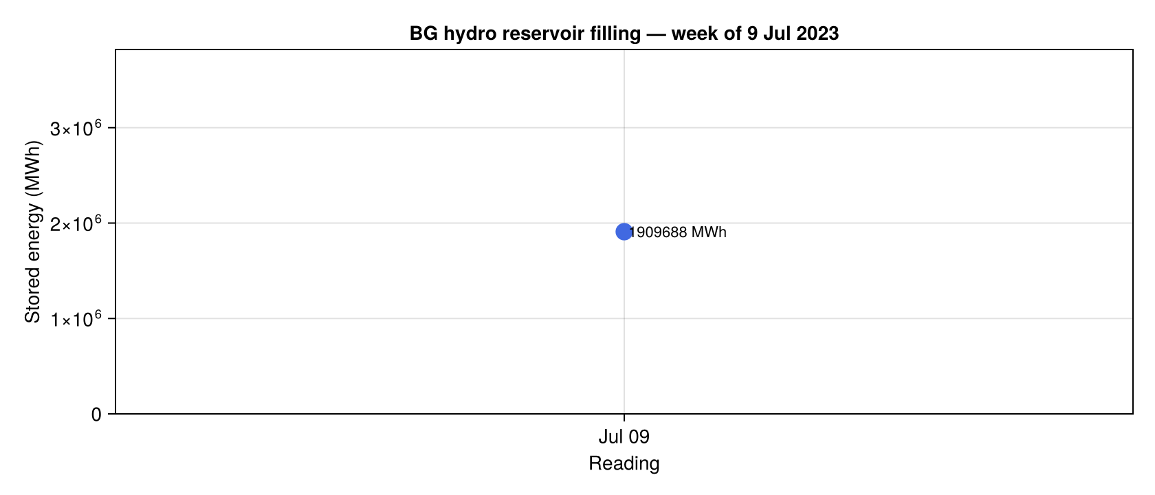

A single weekly reading produces a sparse curve. In practice you'd pull a year of weekly samples — the seasonality of hydro state (drawdown through summer, refill in autumn/winter rains) becomes the headline. Just hand the wrapper the full range and it splits the period into ENTSO-E's one-year windows automatically. You can preview the chunk boundaries the wrapper uses by calling split_period directly:

chunks = split_period(
    DateTime("2020-01-01"), DateTime("2023-01-01"); window = Year(1),
)

3-element Vector{Tuple{Dates.DateTime, Dates.DateTime}}:
 (Dates.DateTime("2020-01-01T00:00:00"), Dates.DateTime("2021-01-01T00:00:00"))
 (Dates.DateTime("2021-01-01T00:00:00"), Dates.DateTime("2022-01-01T00:00:00"))
 (Dates.DateTime("2022-01-01T00:00:00"), Dates.DateTime("2023-01-01T00:00:00"))

The wrapper invokes the endpoint once per (start, stop) pair, re-raises the per-chunk ENTSOEAcknowledgements as skips so a partially populated multi-year fetch still returns whatever data exists, and vcats the results. Override the chunk size by passing window = Month(1) (etc.) — useful when a year hits ENTSO-E's response-size cap.

Hydro PSR types side by side

Even from a synthetic snapshot, the installed-capacity decomposition shows where pumped storage sits in the fleet:

fig2 = Figure(size = (640, 360))
ax = Axis(fig2[1, 1];
    title  = "Hydro PSR types (NL fixture for shape)",
    xlabel = "Installed MW",
    yticks = (1:length(hydro_caps),
        [PSR_LABELS[Symbol(c)] for c in hydro_caps.psr_type]),
)
barplot!(ax, 1:length(hydro_caps), hydro_caps.capacity_mw;
    direction = :x,
    color = [:royalblue, :seagreen, :purple][1:length(hydro_caps)],
    strokewidth = 0.4, strokecolor = :white)
fig2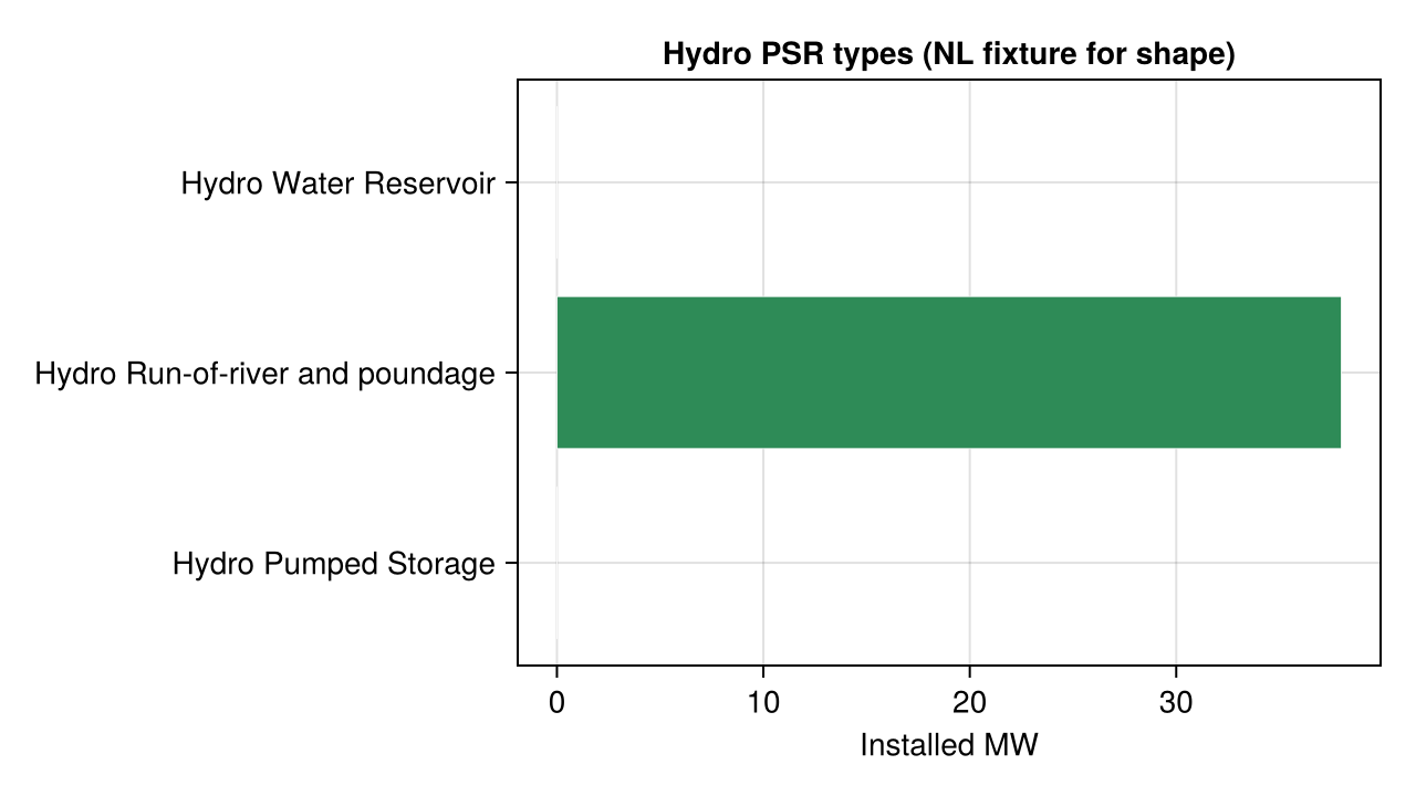

Where to next

• actual_generation_per_production_type with psr_type = PsrType.HYDRO_PUMPED_STORAGE or PsrType.HYDRO_WATER_RESERVOIR for the actual hourly hydro output — pair it with this reservoir state to study drawdown rate.

• Multi-year fetches just work — the wrapper splits the range into the one-year windows ENTSO-E permits. Override the window keyword (window = Month(1)) for finer-grained chunking, or use split_period if you want the window boundaries directly.