Tutorial: a Dutch electricity day in three plots

This page walks through three queries against the ENTSO-E Transparency Platform API and plots the results with CairoMakie.

The HTTP traffic is served from cassettes under test/cassettes/, recorded once with a real API token. That means this page builds offline, on every CI run, with no credentials — exactly the same data every time. To re-record (e.g. against a different date), delete the relevant .yml and re-run the test suite once with ENTSOE_API_TOKEN (or token.txt) set.

We focus on the Netherlands on 2 September 2024 (a normal shoulder-season weekday) for the time-series plots, and NL calendar-year 2024 for the installed-capacity bar chart.

Setup

Build a client and configure BrokenRecord against our committed cassette directory. All three queries below go through the named-argument convenience wrappers (day_ahead_prices, actual_total_load, installed_capacity_per_production_type), which already parse the XML and accept DateTime arguments directly — no hand-written parsing or entsoe_period(...) boilerplate per call.

julia

using ENTSOE
using CairoMakie
using Dates: DateTime

CairoMakie.activate!(type = "png")

# BrokenRecord setup is shared with the test suite — a small helper file
# that loads the package, applies the Julia 1.12 STATE-padding
# workaround, and configures cassette path + token-redacting
# `ignore_query`. Returns the module so we can call `BR.playback(...)`.
include(joinpath(pkgdir(ENTSOE), "test", "_brokenrecord_helpers.jl"))
const BR = _load_brokenrecord()

# Token is irrelevant in playback mode — the HTTP layer is
# intercepted before the request reaches ENTSO-E. Any non-empty
# string lets `ENTSOEClient` build a valid client.
client = ENTSOEClient("PLAYBACK")

Day-ahead electricity prices

day_ahead_prices wraps Market 12.1.D (documentType=A44). It pre-fills both in_Domain and out_Domain to the requested area, normalises the period bounds, and returns a parsed StructVector of (time, value) rows straight away.

julia

prices = BR.playback("market_121d_day_ahead_prices_NL.yml") do
    day_ahead_prices(client, EIC.NL,
        DateTime("2024-09-01T22:00"),
        DateTime("2024-09-02T22:00"))
end
length(prices), prices[1], prices[end]

(24, (time = Dates.DateTime("2024-09-01T22:00:00"), value = 91.24), (time = Dates.DateTime("2024-09-02T21:00:00"), value = 104.0))

The result is Tables.jl-compatible — each column is a real Vector you can pull out without an allocation:

julia

prices.value[1:3]    # ::Vector{Float64}

3-element Vector{Float64}:
 91.24
 94.77
 92.39

If you need the raw XML body (to drop into your own XML walker, archive the response, or debug a parse mismatch), pass Raw() as the trailing argument. The same wrapper now returns a String:

julia

xml = BR.playback("market_121d_day_ahead_prices_NL.yml") do
    day_ahead_prices(client, EIC.NL,
        DateTime("2024-09-01T22:00"),
        DateTime("2024-09-02T22:00"),
        Raw())
end
first(xml, 200)

"<?xml version=\"1.0\" encoding=\"utf-8\"?>\n  <Publication_MarketDocument xmlns=\"urn:iec62325.351:tc57wg16:451-3:publicationdocument:7:3\">\n    <mRID>8c6f96f960dd43d8825846643f939b37</mRID>\n    <revisionNum"

The dispatch is on the singleton type — no Union{StructVector, String} in the inferred signature. Without an explicit format the default Parsed() kicks in.

julia

fig = Figure(size = (900, 380))
ax = Axis(fig[1, 1];
    xlabel = "UTC time",
    ylabel = "EUR / MWh",
    title  = "NL day-ahead prices — delivery day 2024-09-02",
)
lines!(ax, [p.time for p in prices], [p.value for p in prices];
    color = :tomato, linewidth = 2)
hlines!(ax, [0.0]; color = (:black, 0.3), linestyle = :dot)
fig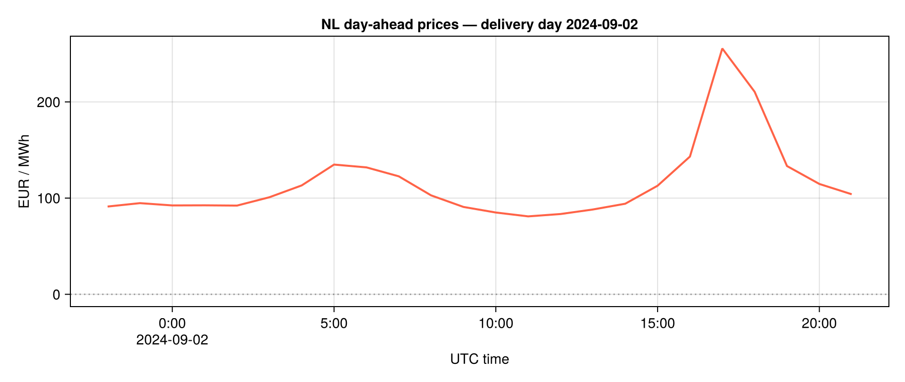

The dip into negative territory in the early afternoon is the characteristic shape of a sunny shoulder-season day on a grid with a lot of solar — wholesale price sags as PV output peaks.

Actual total load

actual_total_load wraps Load 6.1.A (documentType=A65, processType=A16). Quarter-hour resolution, returned as Vector{(time, value)} in MW.

julia

load = BR.playback("load_61a_actual_total_load_NL.yml") do
    actual_total_load(client, EIC.NL,
        DateTime("2024-09-01T22:00"),
        DateTime("2024-09-02T22:00"))
end
length(load), load[1], load[end]

(96, (time = Dates.DateTime("2024-09-01T22:00:00"), value = 12156.45), (time = Dates.DateTime("2024-09-02T21:45:00"), value = 12685.73))

julia

fig = Figure(size = (900, 380))
ax = Axis(fig[1, 1];
    xlabel = "UTC time",
    ylabel = "MW",
    title  = "NL actual total load — delivery day 2024-09-02",
)
lines!(ax, [p.time for p in load], [p.value for p in load];
    color = :steelblue, linewidth = 1.6)
fig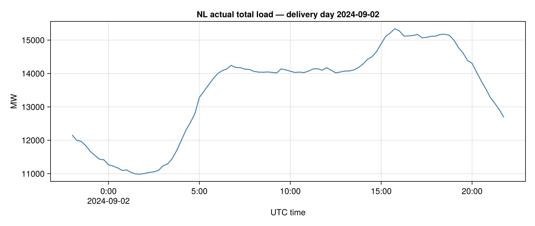

The double-hump morning + evening peak is the typical working-day shape; valley around 02:00–04:00 UTC, ramp-up from ~06:00 as the country wakes up.

Installed capacity by production type

installed_capacity_per_production_type wraps Generation 14.1.A. The returned rows are (psr_type, capacity_mw) — translate the codes to labels with describe against the PSR_LABELS table.

julia

cap_rows = BR.playback("generation_141a_installed_capacity_NL.yml") do
    installed_capacity_per_production_type(client, EIC.NL,
        DateTime("2023-12-31T23:00"),
        DateTime("2024-12-31T23:00"))
end
sort!(cap_rows, by = r -> -r.capacity_mw)
[(ENTSOE.describe(PSR_LABELS, r.psr_type), round(r.capacity_mw; digits = 0))
 for r in cap_rows]

20-element Vector{Tuple{String, Float64}}:
 ("Solar", 27980.0)
 ("Fossil Gas", 18476.0)
 ("Wind Onshore", 6955.0)
 ("Wind Offshore", 4739.0)
 ("Fossil Hard coal", 4012.0)
 ("Waste", 777.0)
 ("Nuclear", 486.0)
 ("Biomass", 418.0)
 ("Hydro Run-of-river and poundage", 38.0)
 ("Other", 1.0)
 ("Fossil Brown coal/Lignite", 0.0)
 ("Fossil Coal-derived gas", 0.0)
 ("Fossil Oil", 0.0)
 ("Fossil Oil shale", 0.0)
 ("Fossil Peat", 0.0)
 ("Geothermal", 0.0)
 ("Hydro Pumped Storage", 0.0)
 ("Hydro Water Reservoir", 0.0)
 ("Marine", 0.0)
 ("Other renewable", 0.0)

julia

labels = [ENTSOE.describe(PSR_LABELS, r.psr_type) for r in cap_rows]
mw     = [r.capacity_mw for r in cap_rows]
fig = Figure(size = (900, 480))
ax = Axis(fig[1, 1];
    xlabel = "MW",
    ylabel = "production type",
    title  = "NL installed capacity by production type — 2024",
    yticks = (1:length(labels), labels),
    yreversed = true,
)
barplot!(ax, 1:length(mw), mw;
    direction = :x, color = :seagreen, strokecolor = :black, strokewidth = 0.5)
fig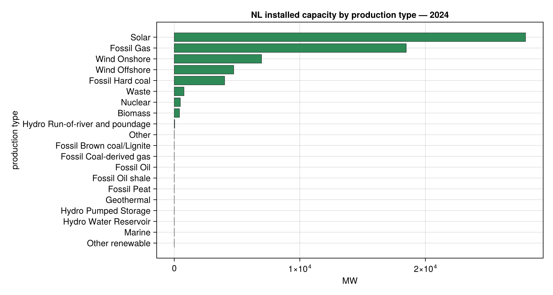

Solar and onshore wind dominate by nameplate, but the capacity-factor story is very different — that's where the load and generation timeseries endpoints come in.

Combined view: load and price on the same window

Plotting load and price on twin axes for the same 24-hour window shows how Dutch wholesale prices respond inversely to net load (solar peak → low residual demand → low price → and vice versa in the evening peak).

julia

fig = Figure(size = (900, 460))
ax1 = Axis(fig[1, 1];
    xlabel = "UTC time",
    ylabel = "MW (load)",
    ylabelcolor = :steelblue,
    title  = "NL load vs day-ahead price — 2024-09-02",
)
ax2 = Axis(fig[1, 1];
    ylabel = "EUR / MWh",
    yaxisposition = :right,
    ylabelcolor = :tomato,
)
hidespines!(ax2)
hidexdecorations!(ax2)

lines!(ax1, [p.time for p in load], [p.value for p in load];
    color = :steelblue, linewidth = 1.6, label = "load")
lines!(ax2, [p.time for p in prices], [p.value for p in prices];
    color = :tomato, linewidth = 2, label = "price")
hlines!(ax2, [0.0]; color = (:black, 0.3), linestyle = :dot)

axislegend(ax1; position = :lt)
fig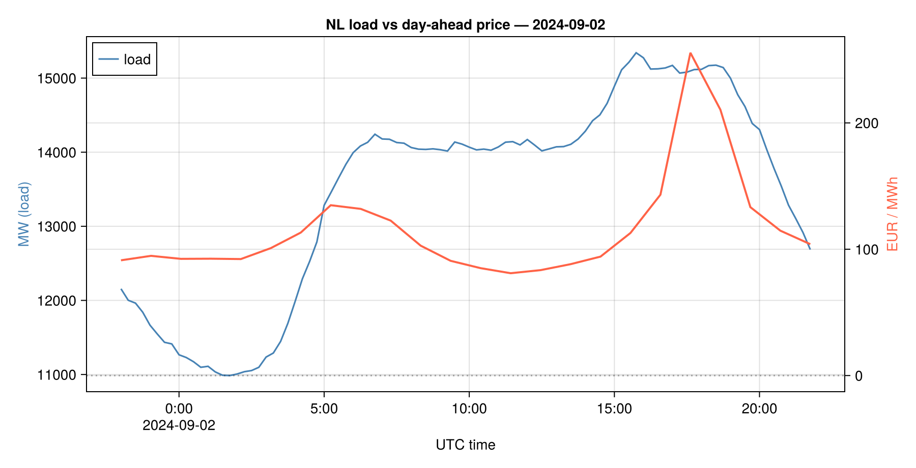

What changed since the last release of this page

Earlier versions of this tutorial shipped ~80 lines of inline XML-walking code — parse_timeseries, parse_installed_capacity, a PSR_LABELS dict — that callers had to copy into their own projects. All of that is now part of the package:

parse_timeseries / parse_timeseries_per_psr / parse_installed_capacity for the two common ENTSO-E document shapes.
PsrType / BusinessType / ProcessType / DocumentType for passing semantically-named codes into wrappers (PsrType.SOLAR == "B16"), and PsrGroup for subset filtering after a fetch.
PSR_LABELS, DOCUMENT_LABELS, PROCESS_LABELS, BUSINESS_LABELS for code → description lookup (used for plot legends, pretty-printing, etc.).
The named-argument wrappers above (one per common endpoint) hide the magic codes and accept DateTime directly.

Drop down to the generated layer (ENTSOE.market121_d_energy_prices, …) only when you need an endpoint we haven't wrapped yet.

Where to next

The full set of generated wrapper functions is in the REST API Reference — each tag page lists every operation with its parameters and a Try-it-out playground.
Browse the Julia-side names (helpers, types, generated functions with their docstrings) on the Generated Reference page.
For very long historical queries you do nothing special: ENTSO-E caps most endpoints at one year per request, and the wrappers split longer ranges into window-sized chunks automatically. See the multi-year tutorial; split_period exposes the chunk boundaries if you need them.
See the cassette mechanism in test/test-cassettes.jl if you want to add fixtures for other endpoints.

Tutorial: a Dutch electricity day in three plots ​

Setup ​

Day-ahead electricity prices ​

Actual total load ​

Installed capacity by production type ​

Combined view: load and price on the same window ​

What changed since the last release of this page ​

Where to next ​

Tutorial: a Dutch electricity day in three plots

Setup

Day-ahead electricity prices

Actual total load

Installed capacity by production type

Combined view: load and price on the same window

What changed since the last release of this page

Where to next